ARIMA(0,1,1) repeating the same point estimate

Question

I have a weekly series stored in a tsibble called data:

data
# A tsibble: 50 x 2 [1W]
         Yw Series
     <week>  <dbl>
 1 2018 W26 0.352 
 2 2018 W27 0.457 
 3 2018 W28 0.435 
 4 2018 W29 0.106 
 5 2018 W30 0.188 
 6 2018 W31 0.226 
 7 2018 W32 0.0769
 8 2018 W33 0.359 
 9 2018 W34 0.194 
10 2018 W35 0.1   
# … with 40 more rows

Using forecast::auto.arima() this is what I get:

> auto.arima(data$Series) %>% summary()


Series: data$Series 
ARIMA(0,1,1) 

Coefficients:
          ma1
      -0.8024
s.e.   0.1175

sigma^2 estimated as 0.01157:  log likelihood=39.72
AIC=-75.43   AICc=-75.17   BIC=-71.65

Training set error measures:
                      ME      RMSE        MAE       MPE     MAPE      MASE      ACF1
Training set -0.01972258 0.1053875 0.08478854 -37.38673 56.40025 0.8320206 0.1053078

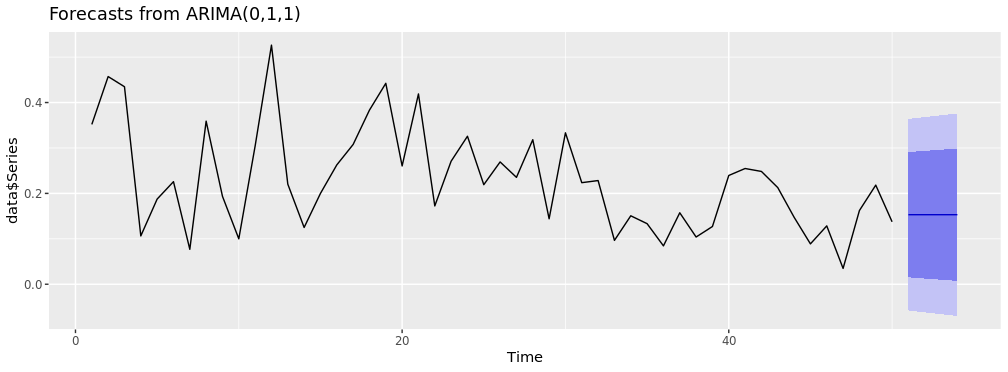
I want to forecast the series for the next month, and it's weekly data, so I ran:

auto.arima(data$Series) %>% 
  forecast::forecast(h = 4) %>% 
  autoplot()

And this is what I get:

Point Forecast       Lo 80     Hi 80       Lo 95     Hi 95
51      0.1530928 0.015248242 0.2909373 -0.05772223 0.3639077
52      0.1530928 0.012584137 0.2936014 -0.06179663 0.3679821
53      0.1530928 0.009969614 0.2962159 -0.06579520 0.3719807
54      0.1530928 0.007402002 0.2987835 -0.06972202 0.3759075

This seems so strange to me. The point estimate is the same for all four weeks ahead and there's no autoregressive component in the model. I've checked and ARIMA(0,1,1) beats all other specifications on both AIC, AICc and BIC.

Can anyone shed some light on this?

Answer 1

So your estimated model is like:

$\Delta_{y_{t+1}}=\beta \epsilon_{t}+\epsilon_{t+1}$ which implies $y_{t+1}=y_{t}+\beta \epsilon_{t}+\epsilon_{t+1}$ where your estimated beta is the value reported in the output of -0.8024. This means that, if you want to predict $y_{t+1}$ given the information set available today at time t, you can do so (as you know the time-t innovation $\epsilon_{t}$), and your prediction on $y_{t+1}$ is $y_{t}+\beta \epsilon_{t}$. In general you can make 1-step-ahead forecasts.

Now, what happens if you want to predict a generic $y_{t+k}$ for k>1? You will have no better prediction that $y_{t+1}$. Indeed $E_{t}(y_{t+2})=E_{t}(y_{t+1}+\beta \epsilon_{t+1}+\epsilon_{t+2})=E_{t}(y_{t+1})=y_{t}+\beta \epsilon_{t}$. This will hold for any k>=2.

Why your auto-specification function is giving you this result? Well, if you have correctly specified the rest of the process distribution and your sample is large enough, then this means that your time series is a I(1) process with very little persistence in the first-difference $\Delta_{y_{t}}$. We could say that it is a touch more persistent than a random walk whose increments are White Noises (because here you have a MA(1) on first differences).

If you want to have a real-world example of similar time-series (i.e. examples of I(1) processes with first diff that are even less persistent than yours on average!), try for example to fit a model like yours on the natural log of daily stock prices. You will see that, for most cases, you will have that even a simple MA(1) on first differences is not significant.