87
$\begingroup$

Even though all the images in the MNIST dataset are centered, with a similar scale, and face up with no rotations, they have a significant handwriting variation that puzzles me how a linear model achieves such a high classification accuracy.

As far as I am able to visualize, given the significant handwriting variation, the digits should be linearly inseparable in a 784 dimensional space, i.e., there should be a little complex (though not very complex) non-linear boundary that separates the different digits, similar to the well-cited $XOR$ example where positive and negative classes can not be separated by any linear classifier. It seems baffling to me how multi-class logistic regression produces such a high accuracy with entirely linear features (no polynomial features).

As an example, given any pixel in the image, different handwritten variations of the digits $2$ and $3$ can make that pixel illuminated or not. Therefore, with a set of learned weights, each pixel can make a digit look as a $2$ as well as a $3$. Only with a combination of pixel values should it be possible to say whether a digit is a $2$ or a $3$. This is true for most of the digit pairs. So, how is logistic regression, which blindly bases its decision independently on all pixel values (without considering any inter-pixel dependencies at all), able to achieve such high accuracies.

I know that I am wrong somewhere or am just over-estimating the variation in the images. However, it would be great if someone could help me with an intuition on how the digits are 'almost' linearly separable.

$\endgroup$
2
  • $\begingroup$ Have a look at the textbook Statistical Learning with Sparsity: the Lasso and Generalizations 3.3.1 Example: Handwritten Digits web.stanford.edu/~hastie/StatLearnSparsity_files/SLS.pdf $\endgroup$
    – Adrian
    Commented Sep 12, 2019 at 18:06
  • $\begingroup$ I've been curious: how well does something like a penalized linear model (i.e., glmnet) do on the problem? If I recall, what you are reporting is the unpenalized out-of-sample accuracy. $\endgroup$
    – Cliff AB
    Commented Sep 13, 2019 at 22:59

2 Answers 2

107
$\begingroup$

tl;dr Even though this is an image classification dataset, it remains a very easy task, for which one can easily find a direct mapping from inputs to predictions.


Answer:

This is a very interesting question and thanks to the simplicity of logistic regression you can actually find out the answer.

What logistic regression does is for each image accept $784$ inputs and multiply them with weights to generate its prediction. The interesting thing is that due to the direct mapping between input and output (i.e. no hidden layer), the value of each weight corresponds to how much each one of the $784$ inputs are taken into account when computing the probability of each class. Now, by taking the weights for each class and reshaping them into $28 \times 28$ (i.e. the image resolution), we can tell what pixels are most important for the computation of each class.

Note, again, that these are the weights.

Now take a look at the above image and focus on the first two digits (i.e. zero and one). Blue weights mean that this pixel's intensity contributes a lot for that class and red values mean that it contributes negatively.

Now imagine, how does a person draw a $0$? He draws a circular shape that's empty in between. That's exactly what the weights picked up on. In fact if someone draws the middle of the image, it counts negatively as a zero. So to recognize zeros you don't need some sophisticated filters and high-level features. You can just look at the drawn pixel locations and judge according to this.

Same thing for the $1$. It always has a straight vertical line in the middle of the image. All else counts negatively.

The rest of the digits are a bit more complicated, but with little imaginations you can see the $2$, the $3$, the $7$ and the $8$. The rest of the numbers are a bit more difficult, which is what actually limits the logistic regression from reaching the high-90s.

Through this you can see that logistic regression has a very good chance of getting a lot of images right and that's why it scores so high.


The code to reproduce the above figure is a bit dated, but here you go:

import tensorflow as tf
import matplotlib.pyplot as plt
from tensorflow.examples.tutorials.mnist import input_data

# Load MNIST:
mnist = input_data.read_data_sets("MNIST_data/", one_hot=True)

# Create model
x = tf.placeholder(tf.float32, shape=(None, 784))
y = tf.placeholder(tf.float32, shape=(None, 10))

W = tf.Variable(tf.zeros((784,10)))
b = tf.Variable(tf.zeros((10)))
z = tf.matmul(x, W) + b

y_hat = tf.nn.softmax(z)
cross_entropy = tf.reduce_mean(-tf.reduce_sum(y * tf.log(y_hat), reduction_indices=[1]))
optimizer = tf.train.GradientDescentOptimizer(0.5).minimize(cross_entropy) # 

correct_pred = tf.equal(tf.argmax(y_hat, 1), tf.argmax(y, 1))
accuracy = tf.reduce_mean(tf.cast(correct_pred, tf.float32))

# Train model
batch_size = 64
with tf.Session() as sess:

    loss_tr, acc_tr, loss_ts, acc_ts = [], [], [], []

    sess.run(tf.global_variables_initializer()) 

    for step in range(1, 1001):

        x_batch, y_batch = mnist.train.next_batch(batch_size) 
        sess.run(optimizer, feed_dict={x: x_batch, y: y_batch})

        l_tr, a_tr = sess.run([cross_entropy, accuracy], feed_dict={x: x_batch, y: y_batch})
        l_ts, a_ts = sess.run([cross_entropy, accuracy], feed_dict={x: mnist.test.images, y: mnist.test.labels})
        loss_tr.append(l_tr)
        acc_tr.append(a_tr)
        loss_ts.append(l_ts)
        acc_ts.append(a_ts)

    weights = sess.run(W)      
    print('Test Accuracy =', sess.run(accuracy, feed_dict={x: mnist.test.images, y: mnist.test.labels})) 

# Plotting:
for i in range(10):
    plt.subplot(2, 5, i+1)
    weight = weights[:,i].reshape([28,28])
    plt.title(i)
    plt.imshow(weight, cmap='RdBu')  # as noted by @Eric Duminil, cmap='gray' makes the numbers stand out more
    frame1 = plt.gca()
    frame1.axes.get_xaxis().set_visible(False)
    frame1.axes.get_yaxis().set_visible(False)
$\endgroup$
6
  • 14
    $\begingroup$ Thanks for the illustration. These weight images make it more clear as how the accuracy is so high. Dot multiplication of a handwritten digit image with the weight image corresponding to the true label of the image does 'seem' to be the highest in comparison to the dot product with other weight labels for most (still 92% look like a lot to me) of the images in MNIST. Still, it's a little surprising that $2$ and $3$ or $7$ and $8$ are seldom misclassified as each other upon examining the confusion matrix. Anyways, this is what it is. The data never lies. :) $\endgroup$ Commented Sep 12, 2019 at 0:27
  • 13
    $\begingroup$ Of course it helps that MNIST samples are centered, scaled, and contrast-normalized before the classifier ever sees them. You don't have to address questions like "what if the edge of the zero actually goes through the middle of the box?" because the pre-processor has already gone a long way towards making all zeroes look the same. $\endgroup$
    – hobbs
    Commented Sep 12, 2019 at 18:41
  • 1
    $\begingroup$ @EricDuminil I added a commend on the script with your suggestion. Thanks a lot for the input! :D $\endgroup$
    – Djib2011
    Commented Sep 13, 2019 at 14:03
  • 1
    $\begingroup$ @NitishAgarwal, If you think that this answer is the Answer to your Question, consider marking it as such. $\endgroup$
    – sintax
    Commented Sep 13, 2019 at 16:02
  • 17
    $\begingroup$ For someone who's interested in but not particularly familiar with this sort of processing, this answer provides a fantastic intuitive example of the mechanics. $\endgroup$ Commented Sep 15, 2019 at 2:29
3
$\begingroup$

Accepted answer is good, but I think there is more to this. It describes a case with cross-entropy loss, but MNIST can be learned with 87% accuracy even with MSE loss.

Here are example digit patterns learned with MSE loss: digits 0-9 patterns

Dot-product input image with all of these patterns, and the biggest dot-product will determine our digit class.

However, those patterns are trained with binarized (0 or 1) pixels, no floating point values. When two patterns in dot-product are binarized, dot-product effectively calculates "common area", the number of 1-pixels which are shared in both vectors. The fact that this "comparing common area" method achieves 87% accuracy implies that images in one class in MNIST dataset overlap a lot.

Still, when we check "average" images for each digit class, they are far from these patterns:

means of MNIST digit classes

These patterns (just means) achieve 64% accuracy on MNIST test set! If I center the pixel values (subtract 0.2 from pixel values), I get 75% accuracy. This is a big argument for "shared area" explanation.

Why original patterns differ so much from mean images, if we compare areas? The reason is that we should calculate weighted average, when in-class images get more weight than images out-class. One easy idea is to weight -1 all out-of-class images, and +1 all in-class images. But because we have more out-of-class images, this will make affect our patterns too negatively for out-of-class, so instead let's do

-mean(out-of-class digits) + mean(in-class digits)

Here are mean(out-of-class digits), yes so similar: enter image description here

and here is difference with mean(in-class digits): enter image description here

Now these patterns look very similar to those from accepted answer, learned with cross-entropy loss!

But we still didn't reproduce original learned patterns. This is because we have chosen very simple weighted means (-1 out-of-class, +1 in-class). In reality each data point (training digit) gets it's own weight coefficient.

Weight coefs for class-0 MNIST digits are: -0.1645, 0.1290, 0.1497, 0.0644, -0.0883, -0.0078, 0.1196, -0.1105, 0.0919, 0.1153, ...

If I add sum MNIST digits using those weights, I get (each image is weighted running sum): enter image description here

Last weight coeffs are: ..., 0.2693, -0.0031, -0.0041, -0.0511, -0.4518, 0.0176, 0.0539, -0.0661, 0.0607, -0.1115. Last running image sums:

enter image description here

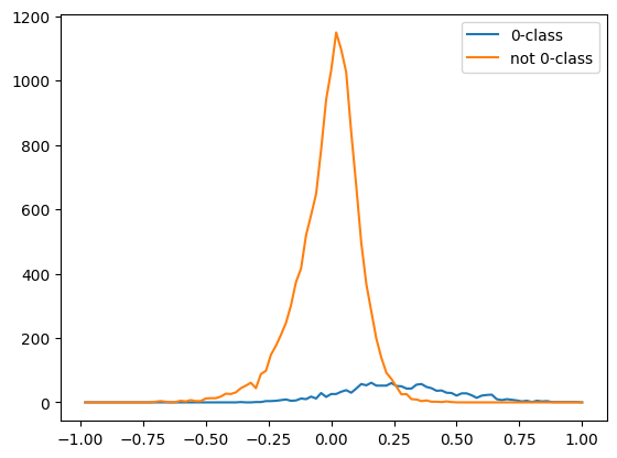
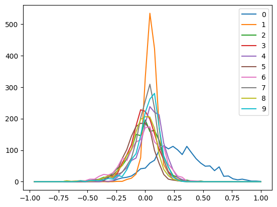
In the end we arrive to original pattern of "0-class", which I posted at the beginning. The coefficients are not always negative for out-of-clas and positive for in-class. Here are distributions of weight coefs values. In-class (in this case, for 0-class) are centered around +0.25, while out-of-class are centered around 0:

enter image description here enter image description here


Bottom line of this: MNIST test digits have a lot of pixel-wise overlap with MNIST train digits. We can figure out digit class by calculating weighted sum of shared areas (shared with training digits). MSE loss learns exactly these patterns, but without calculating weighted coefs directly.

Sometimes it helps to think about this as "just patterns" :)

Coefficients can be calculated by solving MNIST as system of linear equations, as described in here.

$\endgroup$
3
  • 1
    $\begingroup$ This answer is good (+1) but I think the focus on loss functions is misplaced. The difference between MSE and cross-entropy loss is not really material to the big idea, which is that digits are "just patterns," so a model just has to do a trivial amount of "template matching" to correctly identify it. (And, of course, all of the MNIST pre-processing steps to isolate a digit, center it, crop just the digit and adjust the contrast all play a large role in simplifying this task compared to a harder digit task like Street View House Number, and SVHN is still simplified!) $\endgroup$
    – Sycorax
    Commented Oct 17, 2023 at 14:35
  • $\begingroup$ @Sycorax yes, I mentioned MSE loss only because with MSE loss and binarized digits I know how to solve MNIST analytically, get exact coefficients for each digit pattern, and thus "weighted common area" argument holds mathematically. For cross-entropy loss I don't have such analytical solution. $\endgroup$
    – danbst
    Commented Oct 17, 2023 at 14:42
  • 1
    $\begingroup$ That's a perfectly reasonable choice to make for this demonstration, and the visual results are very striking, so the presentation is completely clear. (Really -- I want to upvote a second time!) Just as an aside, though, logistic regression is convex under mild conditions, so determining the optimal coefficients is straightforward optimization, even if you can't directly solve for them. $\endgroup$
    – Sycorax
    Commented Oct 17, 2023 at 14:46

Your Answer

By clicking “Post Your Answer”, you agree to our terms of service and acknowledge you have read our privacy policy.

Not the answer you're looking for? Browse other questions tagged or ask your own question.