The statistical part of this question is unanswerable because the meaning of "best" is not given. (Presumably it occurs in a context of comparing the means of two populations, where minimizing the variance of the difference of two sample means leads to the greatest power to detect a difference.)
The other part--to minimize the variance of the difference of two means--can be solved without Calculus. Indeed, because the sample sizes are integral, Calculus is not necessarily even a good tool for the solution. Using basic principles of arithmetic order and knowledge of how to add fractions, we can identify the limitations of the Calculus-based solution and obtain a universally correct answer.
To establish notation, let $\sigma_1^2 = 8^2$ be the variance of one population and $\sigma_2^2 = 12^2$ be the variance of the other. The question contemplates taking samples of size $n_1$ and $n_2,$ respectively, with $n_1+n_2=n=16+9.$ The variances of the sample means therefore are
$$\operatorname{Var}(\bar x_i) = \frac{1}{n_i}\sigma_i^2,\quad i=1,2,$$
whence (assuming the samples are independent!) the variance of the difference of means is
$$\operatorname{Var}(\bar x_1 - \bar x_2) = \frac{\sigma_1^2}{n_1} + \frac{\sigma_2^2}{n_2} = \frac{\sigma_1^2}{n_1} + \frac{\sigma_2^2}{n - n_1}.\tag{1}$$
The last equality shows that $n_1$ is the sole quantity we are free to vary in order to minimize the variance. Because it is a sample size and because there must be at least one element in each of the two samples, $n_1$ is an integer between $1$ and $n-1$ inclusive. Let's consider what happens to the variance in $(1)$ as we begin at $n_1=1$ and successively increment it to $2, 3, \ldots, n-1.$ The values are
$$\frac{\sigma_1^2}{1} + \frac{\sigma_2^2}{n - 1},\ \frac{\sigma_1^2}{2} + \frac{\sigma_2^2}{n - 2},\ \ldots,\ \frac{\sigma_1^2}{n_1} + \frac{\sigma_2^2}{n - n_1},\ \ldots,\ \frac{\sigma_1^2}{n-1} + \frac{\sigma_2^2}{1}.$$
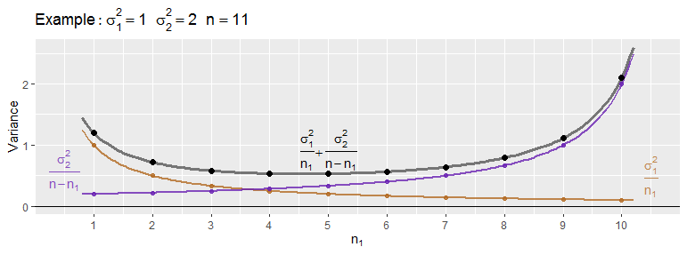
These values are portrayed as the black points in this figure:

Before getting to the question, let's find a solution.
The successive differences
$$\eqalign{
\delta_{n_1} &= \left(\frac{\sigma_1^2}{{n_1}+1} + \frac{\sigma_2^2}{n - ({n_1}+1)}\right) - \left(\frac{\sigma_1^2}{{n_1}} + \frac{\sigma_2^2}{n - {n_1}}\right) \\&= -\frac{\sigma_1^2}{{n_1}({n_1}+1)} + \frac{\sigma_2^2}{(n-{n_1})(n-{n_1}-1)}}$$
give the amounts by which the variance changes as ${n_1}$ is increased to ${n_1}+1.$ Let's analyze them by considering the two terms on the right hand side separately. The denominator of the first, ${n_1}({n_1}+1),$ increases each time ${n_1}$ is incremented because each term in the denominator is positive and increases. Likewise, the denominator of the second decreases each time ${n_1}$ is incremented. This explains why the colored curves (tracking the values of $\sigma_1^2/n_1$ and $\sigma_2^2/n_2$ for real values of $n_1$) must accelerate upward for the first and decelerate downward for the second. Consequently, their sum must be accelerating upward.
We are practically done, because this analysis permits just three possibilities:
The variance $(1)$ increases for every $n_1\ge 1.$ Obviously, then, the minimum is at $n_1=1.$
The variance $(2)$ decreases for every $n_1\ge 1.$ Obviously the minimum is at $n_1=n-1.$
Otherwise, there must be some integer $n_1$ between $1$ and $n-2,$ inclusive, at which the variance $(1)$ stops decreasing and begins increasing. To be precise, the increment from $n_1-1$ to $n_1$ is negative while the increment from $n_1$ to $n_1+1$ is not negative.
Consequently, an optimal value of $n_1$ is attained as $k+1$ where $k$ is the last (largest) value less than $n-1$ for which $\delta_{k}\le 0.$ When $\sigma_1=\sigma_2$ this is a linear equation with solution $(n-1)/2$ and otherwise is a quadratic equation, solvable with the quadratic formula. Exactly one of the roots will lie between $0$ and $n-1.$ Such solutions are generally non-integral and so need to be rounded up (the ceiling function, $\lceil \cdot \rceil$). This yields the following general, correct result for all $n\ge 2:$
When $\sigma_1=\sigma_2,$ set $x = \frac{n-1}{2}.$ Otherwise set $$x = \frac{-(\sigma_2^2 + (2n-1)\sigma_1^2) + \sqrt{(\sigma_1^2+\sigma_2^2)^2 + 4(n^2-1)\sigma_1^2\sigma_2^2}}{2(\sigma_2^2 - \sigma_1^2)}.$$ The optimal value of the variance in formula $(1)$ is attained at $n_1 = \lceil x \rceil.$ When $\delta_{n_1}=0,$ the optimal value is also attained at $n_1=\lceil x \rceil + 1.$
In the example shown in the figure with $\sigma_1^2=1,$ $\sigma_2^2=2,$ and $n=11,$ we find $x=4.064382,$ whence the best sample sizes to use are $n_1=5$ and $n_2=n-n_1=6.$
With the information in the question, $x=9.504166$ giving the solution $n_1=10, n_2=15:$ thus, an optimal sample devotes more observations to the second (higher-variance) group.
Let's now consider the question: it proposes that the optimal value of $n_1$ is
$$n_1^{*} = n\frac{\sigma_1}{\sigma_1+\sigma_2},$$
which entails
$$n_2^{*} = n- n_1^{*} = n\frac{\sigma_2}{\sigma_1+\sigma_2}.$$
This cannot be generally correct, because usually this number is not even an integer and it could easily be less than $1$ or greater than $n-1,$ none of which are valid sample sizes. However, we can still play the increment game by plugging this value for $k=n_1^{*}$ into the formula for $\delta_k$ to see whether the underlying curve in the figure rises or not. Thus:
$$\eqalign{
\delta_{n_1^{*}} &= -\frac{\sigma_1^2}{n_1^{*}\left(n_1^{*}+1\right)} + \frac{\sigma_2^2}{n_2^{*}\left(n_2^{*}-1\right)} \\
&= -\frac{\sigma_1^2}{\left(n\frac{\sigma_1}{\sigma_1+\sigma_2}\right)\left(\left(n\frac{\sigma_1}{\sigma_1+\sigma_2}\right)+1\right)} + \frac{\sigma_2^2}{\left(n\frac{\sigma_2}{\sigma_1+\sigma_2}\right)\left(\left(n\frac{\sigma_2}{\sigma_1+\sigma_2}\right)-1\right)} \\
&= \frac{n\sigma_1\sigma_2(\sigma_1^2 + \sigma_2^2)}{(*)}
}$$
where "$(*)$" denotes the product of the preceding denominators, both of which are positive (in case (3)). This product therefore is clearly positive, making it clear that $\delta_{n_1^{*}}$ is positive, too. But reversing the roles of groups $1$ and $2$ shows that decrementing the value of $\delta_{n_1^{*}}$ is also positive. Consequently,
the optimal sample size $n_1$ must lie within the interval from $n_1^{*}-1$ to $n_1^{*}+1$ (and cannot include either endpoint).
This yields an effective algorithm to find $n_1^{*}$: simply evaluate the variance $(1)$ at the one or two integers that lie in this interval and pick $n_1$ to be a value for which these one or two variances are smallest.
It is possible for there to be two optima. For instance, this always occurs in the commonly-encountered situation where $\sigma_1=\sigma_2$ and $n=2m+1$ is odd. The symmetry between the groups in this situation implies that when $n_1^{*}$ is optimal, so is $n-n_1^{*}.$ Since these numbers must lie within an interval of length two, the two solutions can only be $m$ and $m+1.$ You may pick one of them arbitrarily.
Finally, possibilities (1) and (2) really can occur. They only require that $\sigma_i/(\sigma_1+\sigma_2) \lt 1/n$ for one of the groups $i,$ for then $n_1^{*}$ is either less than $1$ or greater than $n-1.$ These cases may be subsumed in the general algorithm by limiting one's exploration to the integers $1, 2, \ldots, n-1,$ even when the interval $(n_1^{*}-1,n_1^{*}+1)$ includes $0$ or $n.$
These cases have an interesting and useful interpretation: when one of the groups has a sufficiently small standard deviation compared to the other, then the variance of the difference of group means is minimized by taking just a single observation from the small-SD group and devoting the rest of the observational budget to the other group. Normally we don't do this, if only because we are rarely sure about the assumed values of the $\sigma_i.$ It therefore is prudent to take at least two samples from each group in order to estimate their standard deviations. This doesn't change the algorithm in any essential way: simply limit the search for optima to the set $n_1\in \{2,3,\ldots, n-2\}.$

