Checking of Measurement in Grouped Data

Question

My teacher uses the formula below when looking for the median and mode of a grouped data.

$$ median = L_m + c\frac{\frac{n}{2} - F_{m-1}}{f_m} \\ mode = L_m +c\frac{f_m - f_{m-1}}{2f_m-f_{m-1}-f_{m+1}} $$

I am so sorry about the format, I am using the mobile app and have limited access on tools upon writing this.

Where the value of $n/2$ that matches or in range in cumulative frequency of the group data will be the median class.

Where the $f_m$ or highest frequency will be the mode class.

$L_m$ is the lowest class boundary, $c$ is the class width, $F_{m-1}$ is the cumulative frequency that comes before the cumulative frequency of the median class, $f_{m-1}$ is the frequency comes before the highest frequency, $f_{m+1}$ comes after the highest frequency.

I am only showing this as a reference as I found different ways of solving the basic measures of a grouped data.

My question is, is there any possible way of telling whether you got the right answer? A checking or signs that you got it right? The same way how you check the sum by subtracting the sum and the value of one of the summand to get the value of other summand. Thank you so much.

Answer 1

Note that the meaning of $m$ is different in each formula.

• In the formula for the median, $m$ represents the first interval where the relative cumulative frequency reaches a value greater or equal to $50\%$, or, equivalently, the interval where the absolute cumulative frequency $F$ in your notation reaches a value greater or equal to $n/2$. Therefore, $F_{m-1} < \frac{n}{2} \leq F_{m}$, where $m-1$ represents the interval before (to the left of) that one. The absolute (non-cumulative) frequency of that interval is $f_m$.

• In the formula for the mode, and considering equal width intervals, $m$ represents the interval with the highest absolute (non-cumulative) frequency $f_m$. The interval to the left of that one is represented by $m-1$ and the interval to the right is represented by $m+1$. Note, however, that if the intervals have different width, we should use the density $d_j = f_j / c_j$, that is computed as the number of observations in interval $j$ divided by the width of interval $j$ and $m$ will represent the interval with the highest density.

---

Regarding the verification of your computations, a few checkpoints might be useful:

• Of course that the result of the median and the mode must be between the lower bound of the first interval and the higher bound of the last interval.

• Both the median and the mode must lie inside the respective closed chosen interval $m$, i.e., they must be in $[L_m; L_m + c]$. This means that when computing each fraction (that latter will be multiplied by $c$) we will get a value in $[0; 1]$.

• Neither the median nor the mode will belong to an interval with zero frequency $f_m$.

• If you plot a cumulative frequency polygon see the figure on the right, you can get an approximate value of the median by drawing an horizontal line at height $n/2$ until it intercepts with the polygon. The abscissa $x$ of the interception point is the value of the median.

• If you plot an histogram and draw a segment line between the top right corner of the highest bar and the top right corner of the bar on its left, and another segment line between the top left corner of the highest bar and the top left corner of the bar on its right, the abscissa $x$ of interception point is the value of the mode. See an example.

Answer 2

My interpretation is that by 'right answer' you don't mean whether you computed the formula correctly, but whether correct answers from the formulas match the median and mode of the sample or of the distribution from which the sample was drawn.

Sample. The median of a sample is the middle value of the sorted data for samples of odd size and the average of the middle two values for samples of even size. If you have the actual sample values (before binning) that is easy enough to find. For a sample with tied observations the mode is defined as the most frequently occurring value (if there is one). But for samples from a continuous distribution (where any ties occur only by rounding), I know of no 'official' definition of the mode of a sample, but more on that later.

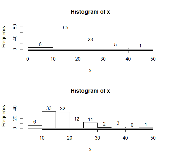
Here are two histograms of the same dataset of size $n=100$ with somewhat different choices of intervals. Accordingly, your formulas will give somewhat different answers. [From your formula, I got about 16 and about 15, respectively. You can use the counts atop histogram bars to check my answers.] The true median of the 100 observations is 16.52 (rounded to 2 places). The modal interval is $(10,20]$ in the top histogram and $(10,15]$ in the bottom histogram, so your formulas will be looking for the 'mode' of the sample in two different intervals. [From your formula, I got roughly 15 for the mode from both histograms.]

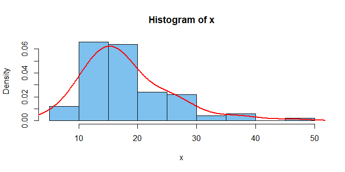
A histogram is one way to get a rough idea of the shape of a population density function, and your formula tries to give a value for the mode that matches that density function. Usually, a somewhat more accurate method is to use a kernel density estimator (KDE). The figure below shows a the second histogram of the data along with the KDE from R statistical software. By looking at the KDE a little more closely, we can find that its maximum value is at about 15.3.

hist(x, prob=T, col="skyblue2")
lines(density(x, adj=1.5), col="red", lwd=2)

Population. If you know the CDF $F$ of the population, then the median is the $x$-value where $F(x)=1/2.$ If you know the density function $f$ of the population, then the mode is the $x$-value that maximizes $f(x),$ if there is a unique maximum.

For example the distribution $\mathsf{Beta}(\text{shape}=\alpha=6, \text{rate}=\beta=1/3)$ has mode $(\alpha - 1)/\beta = 15$ and, by numerical integration, the median is very nearly $17.01.$ [For more on beta distributions, see Wikipedia.]

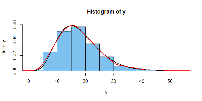
Of course, if the goal is to use a sample to estimate the median and mode of a population, a larger sample will tend to give better results than a smaller one. The figure below shows a histogram of a sample of size $n=2000$ from $\mathsf{Beta}(6,\,1/3),$ along with the population density function (black), and the KDE of the sample (red).