6
$\begingroup$

I have a list of weighted 2D points taken from symmetry analysis of a human back surface. I am supposed to find the "midline" representing the most likely path describing vertebrae location (actually, spinal process of the vertebrae).

EDIT: A representative dataset is as follows:

[[ -0.7898176   -3.35201728   4.36142086]
 [  2.99221402  -3.35201728   1.11907575]
 [  6.97475149  -3.35201728   2.4320322 ]
 [ -4.82443609  -2.35201728   0.6479064 ]
 [ -1.32418909  -2.35201728   1.88004944]
 [  0.07067882  -2.35201728   1.10982834]
 [  3.09169448  -2.35201728   1.8557436 ]
 [  7.10399403  -2.35201728   2.03906224]
 [ -3.07207606  -1.35201728   0.35500973]
 [  2.63202993  -1.35201728   5.32397834]
 [  5.19884868  -1.35201728   1.63816326]
 [  7.65721835  -1.35201728   1.13843392]
 [  2.48172754  -0.35201728   6.65584512]
 [  6.0905911   -0.35201728   1.15552652]
 [  8.62497546  -0.35201728   0.30407144]
 [ -4.7300089    0.64798272   0.31481496]
 [ -3.03274093   0.64798272   0.95337568]
 [  2.19653614   0.64798272  10.3675204 ]
 [  6.20384058   0.64798272   1.42106077]
 [ -4.08636605   1.64798272   0.28875288]
 [  2.03344989   1.64798272  13.04648211]
 [ -4.11717795   2.64798272   0.39713141]
 [  1.93304283   2.64798272  10.41313242]
 [ -4.37994815   3.64798272   0.84588643]
 [  1.66081408   3.64798272  14.96380955]
 [ -4.19024027   4.64798272   0.73216113]
 [  1.60252433   4.64798272  14.72419286]
 [  6.77837359   4.64798272   0.6186005 ]
 [ -4.14362668   5.64798272   0.93673165]
 [  1.55372968   5.64798272  12.9421123 ]
 [ -4.62223541   6.64798272   0.6510101 ]
 [  1.527865     6.64798272  10.80209351]
 [  6.86820685   6.64798272   0.82550801]
 [ -4.68259732   7.64798272   0.45321369]
 [  1.36167494   7.64798272   6.45338514]
 [ -5.19205787   8.64798272   0.23935013]
 [  1.21003466   8.64798272  10.13528877]
 [  7.6689546    8.64798272   0.32421776]
 [ -5.36436818   9.64798272   0.79809416]
 [  1.26248534   9.64798272   7.67036253]
 [  7.35472418   9.64798272   0.92555691]
 [ -5.61723652  10.64798272   0.4741007 ]
 [  1.23101086  10.64798272   7.97064105]
 [ -7.83024735  11.64798272   0.47557318]
 [  1.20348982  11.64798272   8.20694816]
 [  1.14422758  12.64798272   9.26244889]
 [  9.18164464  12.64798272   0.72428381]
 [  1.0827069   13.64798272  10.08599118]
 [  6.80116007  13.64798272   0.4571425 ]
 [  9.384236    13.64798272   0.42399893]
 [  1.04053491  14.64798272  10.48370805]
 [  9.16197972  14.64798272   0.39930227]
 [ -9.85958581  15.64798272   0.39524976]
 [  0.9942501   15.64798272   8.39992264]
 [  8.07642416  15.64798272   0.61480371]
 [  9.55088151  15.64798272   0.54076473]
 [ -7.13657331  16.64798272   0.32929172]
 [  0.92606211  16.64798272   7.83597033]
 [  8.74291069  16.64798272   0.74246827]
 [ -7.20022443  17.64798272   0.52555351]
 [  0.81344517  17.64798272   6.81654834]
 [  8.52844624  17.64798272   0.70543711]
 [ -6.97465178  18.64798272   1.04527813]
 [  0.61959631  18.64798272  10.33529022]
 [  5.733054    18.64798272   1.2309691 ]
 [  8.14818453  18.64798272   1.37532423]
 [ -6.82823664  19.64798272   2.0314052 ]
 [  0.56391636  19.64798272  13.61447357]
 [  5.79971126  19.64798272   0.30148347]
 [  8.01499476  19.64798272   1.72465327]
 [ -6.78504689  20.64798272   2.88657804]
 [ -4.79580634  20.64798272   0.36201975]
 [  0.548376    20.64798272   7.8414544 ]
 [  7.62258506  20.64798272   1.52817905]
 [-10.50328534  21.64798272   0.90358671]
 [ -6.59976138  21.64798272   2.62980169]
 [ -3.71180255  21.64798272   1.27094175]
 [  0.5060743   21.64798272  11.06117677]
 [  4.51983105  21.64798272   1.74626435]
 [  7.50948795  21.64798272   3.46497629]
 [ 11.10199877  21.64798272   1.78047269]
 [-10.15444935  22.64798272   1.47486166]
 [ -6.26274479  22.64798272   4.73707852]
 [ -3.45440904  22.64798272   1.72516012]
 [  0.52759064  22.64798272  12.58470433]
 [  4.22258017  22.64798272   2.63827535]
 [  7.03480033  22.64798272   3.506412  ]
 [ 10.63560314  22.64798272   3.56076386]
 [ -5.95693623  23.64798272   2.97403863]
 [ -3.66261423  23.64798272   2.31667236]
 [  0.52051366  23.64798272  12.5526344 ]
 [  4.21083787  23.64798272   1.95794387]
 [  6.82438636  23.64798272   4.77995659]
 [ 10.18138299  23.64798272   5.21836205]
 [ -9.94629932  24.64798272   0.4074823 ]
 [ -5.74101948  24.64798272   2.60992238]
 [  0.52987226  24.64798272  10.68846987]
 [  6.29981921  24.64798272   3.56204471]
 [  9.96431168  24.64798272   2.85079129]
 [ -9.64229717  25.64798272   0.4503241 ]
 [ -5.579063    25.64798272   0.64475469]
 [  0.52053534  25.64798272  10.05046667]
 [  5.79167815  25.64798272   0.92797027]
 [ 10.05116919  25.64798272   2.52194933]
 [ -8.55286247  26.64798272   0.94447148]
 [  0.45065604  26.64798272  10.97432823]
 [  5.50068393  26.64798272   2.39645232]
 [ 10.08992273  26.64798272   2.77716257]
 [-16.62381217  27.64798272   0.2021621 ]
 [ -9.62146213  27.64798272   0.62245778]
 [ -7.66905507  27.64798272   2.84466396]
 [  0.38656111  27.64798272  10.74369366]
 [  5.76925402  27.64798272   1.13362978]
 [  9.83525197  27.64798272   1.18241147]
 [-15.64874512  28.64798272   0.18279302]
 [ -7.52932494  28.64798272   2.94012191]
 [  0.32171219  28.64798272  10.73770466]
 [  9.4062684   28.64798272   1.41714298]
 [-12.71287717  29.64798272   0.70268073]
 [ -7.59473877  29.64798272   2.16183026]
 [  0.20748772  29.64798272  12.97312987]
 [  3.92952496  29.64798272   1.54987681]
 [  9.05148017  29.64798272   2.40563748]
 [ 14.96021523  29.64798272   0.55258241]
 [-12.14428813  30.64798272   0.36365363]
 [ -7.12360666  30.64798272   2.54312163]
 [  0.40594038  30.64798272  12.64839117]
 [  4.59465757  30.64798272   1.23496581]
 [  8.54333134  30.64798272   2.18912857]
 [-10.6296531   31.64798272   1.4839259 ]
 [ -7.09532763  31.64798272   2.0113838 ]
 [  0.37037733  31.64798272  12.2071139 ]
 [  3.01253349  31.64798272   3.01591777]
 [  4.64523695  31.64798272   3.50267541]
 [  8.39369696  31.64798272   2.53195817]
 [ -7.07947026  32.64798272   1.01324147]
 [  0.39269437  32.64798272   9.67368625]
 [  8.58669997  32.64798272   1.00475646]
 [ 12.02329114  32.64798272   0.50782399]
 [-10.13060786  33.64798272   0.31475653]
 [ -7.30360407  33.64798272   0.35065243]
 [  0.49556923  33.64798272   9.66608818]
 [ -5.37822311  34.64798272   0.38727401]
 [  0.4958055   34.64798272   7.5415026 ]
 [  6.07719006  34.64798272   0.63012453]
 [ -4.64579055  35.64798272   0.39990249]
 [  0.46323666  35.64798272   4.60449213]
 [  4.72819312  35.64798272   0.98050594]
 [ -4.62418372  36.64798272   0.64160709]
 [  0.48866236  36.64798272   4.29331656]
 [  5.06493722  36.64798272   0.59888608]
 [  0.49730481  37.64798272   1.32828464]
 [ -1.31849217  38.64798272   0.70780886]
 [  1.70966455  38.64798272   0.88052135]
 [  0.06305774  39.64798272   0.47366487]
 [  2.13639356  39.64798272   0.67971461]
 [ -0.84726354  40.64798272   0.63787522]
 [  0.55723562  40.64798272   0.62855097]
 [  2.22359779  40.64798272   0.33884894]
 [  0.77309816  41.64798272   0.4605534 ]
 [  0.56144565  42.64798272   0.43678788]]

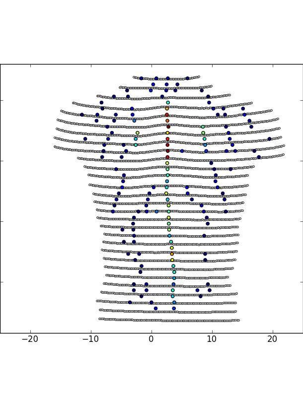
When plotted, my pointcloud typically looks like this, with color representing the "fitness" of a point (how much its neighbourhood is symmetric according to a certain criterion):
enter image description here

EDIT: the colored points are obtained as follows:

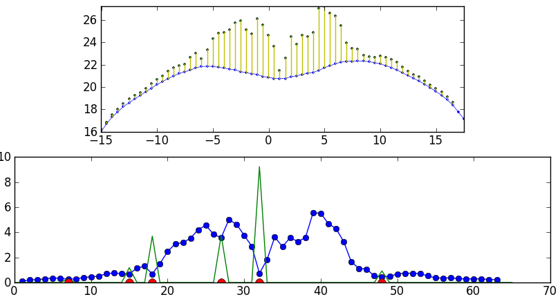
  1. For each horizontal level (points with same Y coordinate) an almost horizontal slice is taken from the back surface model. For each point in this slice, a tangent is drawn and the slice is divided in right side and left side. Then, the difference between the distances of each bilateral pair of points to that line is measured and summed. Then, for each point we have a weight that tells how much the right side and the left side of the slice at that point are equal. The images below illustrate it:

Graph showing a slice of the back surface at the lumbar level, where each point receives a value for its asymmetry. The local minima are selected (red points) with a weight (green triangles) proportional to how much it is "better" than its vicinity (how deep its asymmetry value is, locally).
enter image description here

I am wondering which fitting/regression method should I use, in order to get:

  • Local differentiability (could be approximated);
  • Ability to interpolate to arbitrary resolution;
  • No overshoot or unpredictable oscillations;
  • If possible, outlier removal.

I suspect something might be done with least-squares, radial basis functions, RANSAC, etc. but I also suspect I don't have enough knowledge to select a proper method, so that's why I'm asking the experts.

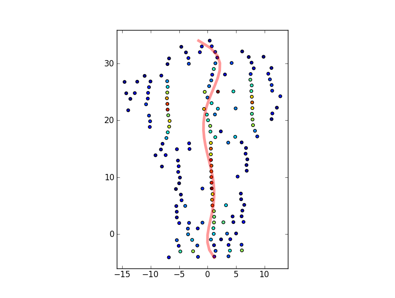
EDIT: performing a weighted spline interpolation, I get results similar to the one below, but it is too sensitive to "outliers", and subject to oscillations obviously far away from what should be the "right" central line:
enter image description here

Any help is much welcome, thanks for reading"

$\endgroup$
9
  • $\begingroup$ @whuber Actually the points to consider are just the colored circles. The gray dots are just there to provide a reference frame of the human torso, and belong to another dataset. The colored points are stored in a matrix of N (x,y) coordinates, with shape Nx2. By differentiability I mean to be able to find the tangent (slope) of the interpolated curve for a given Y coordinate. $\endgroup$ Commented Nov 8, 2012 at 13:58
  • $\begingroup$ Have you considered using a model that would actually be related to the physics of the problem? For example, you could think of modelling the spine as a worm-like chain: en.wikipedia.org/wiki/Worm-like_chain $\endgroup$
    – Bitwise
    Commented Nov 8, 2012 at 14:53
  • $\begingroup$ @whuber The red line is actually a "wrong" fit given by a naive weighted spline interpolation. The color of the dots mean the weight of each point. This weight is calculated by a function which analyzes the local symmetry around the given point. Points which have very similar shapes on both sides have a high simmetry and are heuristically more likely to lie in the midline of the back surface. $\endgroup$ Commented Nov 8, 2012 at 15:32
  • $\begingroup$ @Bitwise Thanks for the link, I'm gonna take a look at it! $\endgroup$ Commented Nov 8, 2012 at 15:33
  • 1
    $\begingroup$ @whuber I'll paste a sample original surface data and some python code to render it. It is a line-structured point cloud over which I perform interpolation with scipy.interpolate.rbf (not included for now). $\endgroup$ Commented Nov 9, 2012 at 21:24

2 Answers 2

4
$\begingroup$

(assuming you want to use python)

The easiest (given what's currently available) would be to use a polynomial and robust methods from statsmodels.

something like

endog = y  # observed points, one dimensional array
#polynomial array as explanatory variable:
#assuming x contains the vertical points
x = x / float(x.max() - x.min()) * 2 - 1 #optional rescaling 
exog = np.vander(x, 5) 

import statsmodels.api as sm
#robust estimation
res = sm.RLM(endog, exog).fit()
print res.summary()
poly = np.poly1d(res.params)
#now we have a polynomial, and we can use differentiation, ... with it

I just typed this, and didn't run it. Also I don't know what order of the polynomial would be useful in this case.

I would use, chebvander from numpy.polynomial, but I don't remember the details, especially handling the shift in domain.

RLM.fit has several different options, if the "outliers" or large spread of points are not handled correctly with the default. http://statsmodels.sourceforge.net/stable/rlm.html

Quantile regression would be a good alternative to RLM. Someone contributed a script for it for statsmodels, but it is not included yet. quantile regression could be used to estimate a "median line" that might work well in this case.

Fitting splines instead of polynomials might be better, but it's not available in python without a bit of work, and I think it will not make much difference given the relatively small number of vertical points.

update:

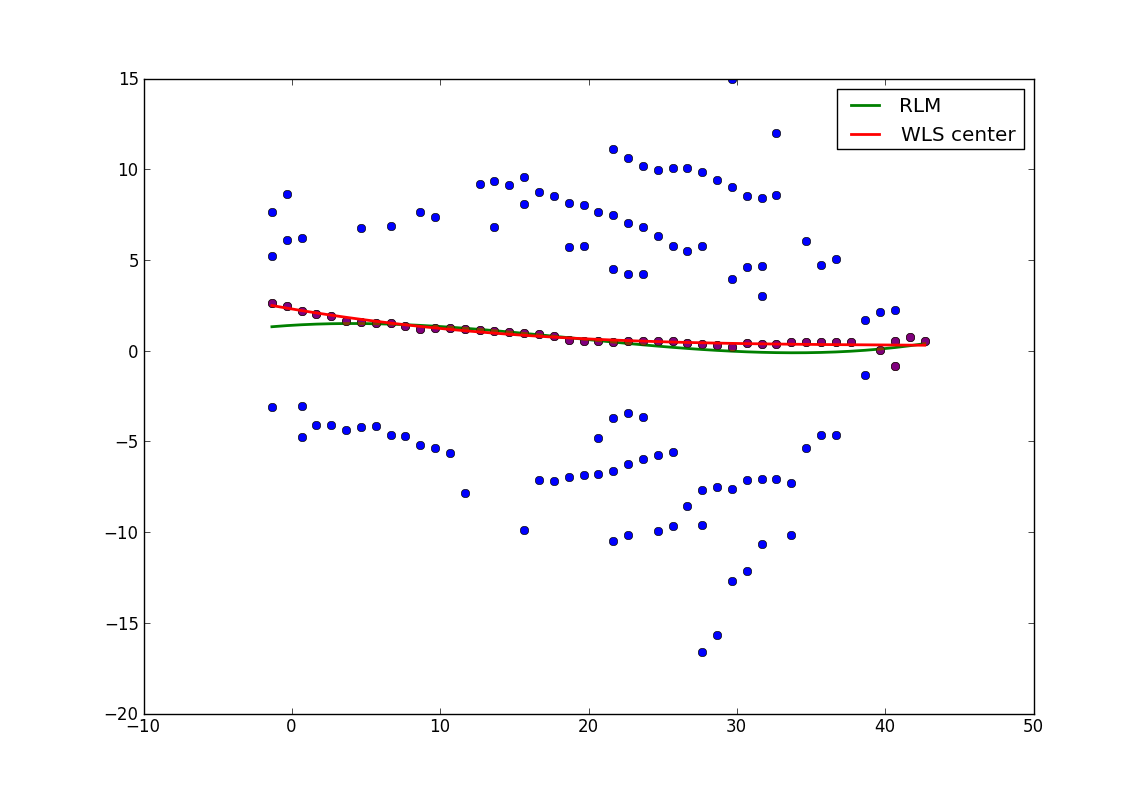
using the data from columns 0 and 1, I tried out RLM. I didn't manage to get the obvious options for RLM to work, but there are still some more uncommon options that I haven't tried.

What I tried instead was to put directly all the weight on the center points. This is essentially least trimmed squares, with an initial robust (M-) estimation of the center points. The first stage fits a low order polynomial. Then we select points with a small residual. I selected the threshold manually to get the right points. Then I fit a higher order polynomial with weighted least squares and put weight only on the center points.

2 stage fitting, with WLS on centerpoints only

This seems to work for estimating the line for the center points, but I don't know yet how this would perform for more general problems.

Except for importing numpy and matplotlib.pyplot and for loading the data, my script to produce the graph is:

#use data in column 1
#rescaling didn't matter much
d = 0.1
x_rs = a[:,1]  #a is original data
x_rs = (x_rs - x_rs.min())
x_rs = x_rs / x_rs.max() #* (1-d) *2 - 1 + d
print x_rs.min(), x_rs.max()

degree = 3  #preliminary regression
exog = x_rs[:,None] ** np.arange(degree+1)
degree2 = 6  #trimmed regression
exog2 = x_rs[:,None] ** np.arange(degree2+1)

endog = a[:,0]

import statsmodels.api as sm
#fit low order polynomial with robust estimator
res = sm.RLM(endog, exog).fit()

#fit on center points, threshold 1.31 chosen by inspection of residuals
resw = sm.WLS(endog, exog2, weights=(np.abs(res.resid) < 1.31)).fit()

plt.plot(a[:,1], a[:,0], 'o')
plt.plot(a[:,1], res.fittedvalues,  '-', lw=2, label='RLM')
idx = np.nonzero(np.abs(res.resid) < 1.31)[0]
plt.plot(a[idx,1], a[idx,0], 'ro', alpha=0.5)
plt.plot(a[:,1], resw.fittedvalues,  '-', lw=2, label='WLS center')
plt.legend()

plt.show()

update 2

One problem with the options for robust estimation is how much control we have over the variance estimate. RLM updates the variance and in this case it downweights the outlying observations not enough.

If we have a prior estimate of the variance, then we can force RLM to use it and not to update it.

The variance estimate by the trimmed least squares, WLS above, is only about 0.014. If we use this information,

scale = resw.scale
resw2 = sm.RLM(endog, exog2).fit(init=dict(scale=scale), update_scale=False)

then the fitted curve looks very similar to the WLS curve above, although the parameter estimates for the polynomial are different.

(Caveat: This doesn't work yet in statsmodels, the init option is only available in a branch where I worked on robust estimation and improvements to RLM.)

$\endgroup$
7
  • $\begingroup$ That seems promising. I am not at work now, but in a few hours I'm gonna make some tests and post some feedback. Thanks for now! $\endgroup$ Commented Nov 8, 2012 at 15:36
  • $\begingroup$ I ran your code and the results were poor, probably because it is still not properly tuned. I run code from the statsmodels RLM examples and the appear to work for what I need to achieve. I am curious: why did you use np.vander? Does it have to do with the degree of the desired polynomial? Thanks again! $\endgroup$ Commented Nov 8, 2012 at 19:03
  • $\begingroup$ about np.vander : yes, it's essentially the same as x[:,None]**np.arange(degree) (degree=order+1, I think np.vander has columns reversed.) Chebychev polynomials would be better, since they are orthogonal. Did you try a low order polynomial first to see whether it works. $\endgroup$
    – Josef
    Commented Nov 9, 2012 at 1:04
  • $\begingroup$ About RLM: the default parameters are defined, as usual, with the normal distribution plus outliers as the reference case. I haven't seen data like yours yet, so I don't know which options for robust estimation would produce the best results. (maybe concentrated weights in the center and then flat weights from there.) $\endgroup$
    – Josef
    Commented Nov 9, 2012 at 1:20
  • $\begingroup$ Your last example (using my provided sample points) shows a result which represents very much what I was hoping to find. I'm gonna try it with the whole set of points, study the concept of least-trimmed-squares (which I didn't knew), and post some feedback soon after. Thanks again, you've been of much help! $\endgroup$ Commented Nov 9, 2012 at 13:48
0
$\begingroup$

This is an old post but here's a paper worth considering:

"Multidimensional curve fitting to unorganized data points by nonlinear minimization", Lian Fang and David C Gossard

http://www.cs.jhu.edu/~misha/Fall05/Papers/fang95.pdf

And for unordered points this paper is interesting. It describes a method of finding the order of points that are natural neighbors of each other: "Point Ordering with Natural Distance Based on Brownian Motion", Philsu Kim1 and Hyoungseok Kim2

http://downloads.hindawi.com/journals/mpe/2010/450460.pdf

$\endgroup$

Your Answer

By clicking “Post Your Answer”, you agree to our terms of service and acknowledge you have read our privacy policy.

Not the answer you're looking for? Browse other questions tagged or ask your own question.