How to interpret Residuals vs. Fitted Plot

Question

I am investigating the effects of weather on restaurant demand. Currently, I am testing the model assumptions for my multiple linear regression model.

My model specification (simplified) is as follows: lm(Visitor ~ Temperature + Temperature_Squared + Pressure + Clouds + Sun + Rain + Day_Fri + Day_Sat + Day_Sun + Day_Mon + Day_Tue + Day_Wed + Hour_00 + Hour_01 + Hour_02 + Hour_13 + Hour_14 + Hour_15 + Hour_16 + Hour_17 + Hour_18 + Hour_19 + Hour_20 + Hour_21 + Hour_22 + Hour_23 + Holiday, data=dat)

After running the model, I obtained the following two graphs:

1. The residuals vs. fitted plot appears to be relatively flat and homoskedastic. However, it has this odd cutoff in the bottom left, that makes me question the homoskedasticity. What does this plot signal and, more importantly, what does it mean for my interpretation? Is multiple linear regression the correct model?

2. How do I interpret the "bump" in the top-right part of the QQ plot?

NB: The data is complete and does not have unreasonable outliers. Initial results indicate only 1 (out of 6) IVs to be significant, while all control variables are significant. Also, no issues with multicollinearity were detected.

Answer 1

Both the cutoff in the residual plot and the bump in the QQ plot are consequences of model misspecification.

You are modeling the conditional mean of the visitor count; let’s call it $Y_{it}$. When you estimate the conditional mean with OLS, it fits $E(Y_{it}\mid X_{it})=\alpha+\beta X_{it}$. Notice that this specification assumes that if $\beta>0$, you can find a low enough $X_{it}$ that pushes the conditional mean of the visitor count into the negative region. This however cannot be the case in our everyday experience.

Visitor count is a count variable and therefore a count regression would be more appropriate. For example, a Poisson regression fits $E(Y_{it}\mid X_{it})=e^{\alpha+\beta X_{it}}$. Under this specification, you can take $X_{it}$ arbitrarily far towards negative infinity, but the conditional mean of the visitor count will still be positive.

All of this implies that your residuals can't by their nature be normally distributed. You seem to not have enough statistical power to reject the null that they are normal. But that null is guaranteed to be false by knowing what your data are.

The cutoff in the residual plot is a consequence of this. You observe the cutoff because for low predicted (fitted) visitor counts the prediction error (residual) can only get so low.

The bump at the end of your QQ plot also follows from this. OLS underpredicts in the right tail because it assumes that the relationship between $X_{it}$ and the outcome is linear. Poisson would assume it is multiplicative. In turn, the right tail of the residuals in the misspecified model is fatter than that of the normal distribution.

I think @BruceET is making a good point that a “wobble” is natural for any estimator, and the question is whether the wobble is outside of a valid confidence bound. But in this case it also signals model misspecification.

Answer 2

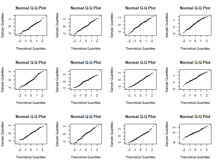
Here are a dozen normal probability plots in R, each for a sample of size 100 from a known standard normal population. Each plot is roughly linear, but most have a 'wobble' or two, especially toward the extremes.

set.seed(116)
par(mfrow=c(3,4))
 for(i in 1:12) {
  z = rnorm(100); qqnorm(z, pch=20) }
par(mfrow=c(1,1))

Repeat the code (without the set.seed statement) for more examples. Examples of normal probability plots in textbooks seem, on average, to be better behaved than the plots one typically sees in practice -- even when normality assumptions are very nearly true.

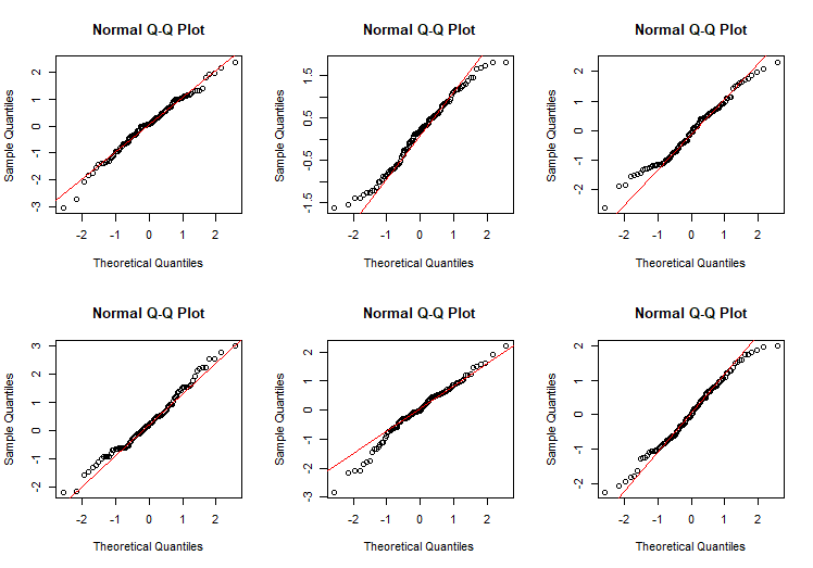
Addendum: Six additional plots with reference lines as suggested in Comment by @Henry.

set.seed(117)
par(mfrow=c(2,3))
 for(i in 1:6) {
  z = rnorm(100)
  qqnorm(z); qqline(z, col=2) }
par(mfrow=c(1,1))

Answer 3

Let's assume "visitors" is the total number of visitors and thus whole positive numbers. Let us assume, the model predicts zero visitors and there are zero visitors,then the residual is zero. If there are more then zero visitors, the the residuals must be positive. If the modell predicts a negative number of visitors, then the residual must be at least of absolute value as the prediction.

In general: as the visitors are bound to a positive or zero value, there is a lower limit to the residuals.

The bump in the QQ plot is minimal and probably not worth worrying about with regards to regression assumptions.