calculate R² as a function of μ,σ

Question

Suppose I fit the sum of $t$ iid random variables

$$y_t=\sum_{i=1}^t{x_i} \space \space \space\space\space x_i \text{ i.i.d} \sim N[\mu,\sigma]$$ to a linear regression model

$$f_t=a\space t +b$$

then I calculate the coefficient of determination $R^2$

$$R^2=RSQ([y_1..y_n],\space [f_1..f_n])$$

I expect that on average $R^2$ will depend on $\mu$ and $\sigma$: $$E[R^2]=f(μ,σ)$$

does such a relationship exist? What is the function $f()$?

Answer 1

What defines $R^2$ in a random walk

As indicated in the comments the process you describe is not appropriate for $R^2$. I have done a simulation (code at bottom) of a random walk using a normal distribution in a linear model - you can tweak the various settings to see what impact they have. We will examine the behaviour now.

Here's what 1000 random walks over 5000 intervals for normally distributed changes with a mean interval change of 1 and a standard deviation of 1. To tweak these simply adjust 'mu' and 'sd' in the code.

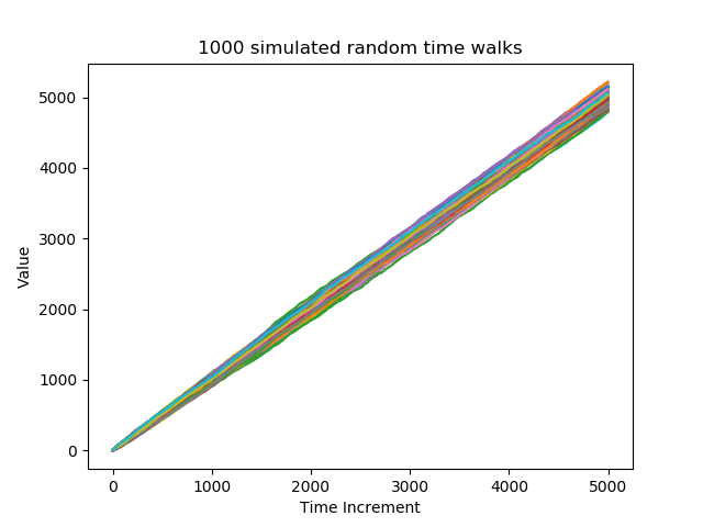
This looks intuitively like you suggestion would work - the lines show upward trends that could be fitted with a linear model. The variation between samples (dispersion) for each interval varies against interval as follows:

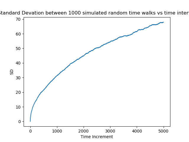
You can see that the variance between interval rises with the number of intervals, which is the central concern underpinning the initial comments to the question. The actual variance is dependent on the interval you look at, so you can get what every answer you want by adjusting your interval range. What about $R^2$ itself? We look at the individual samples and the mean across the samples:

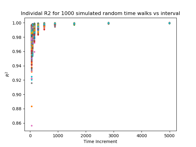$R^2$ for individual trends"> The variation in $R^2$ is dependent on time interval range

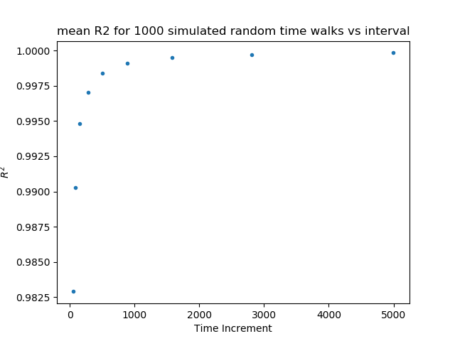$R^2$ across samples"> The mean $R^2$ is very dependent on time interval range

So all in all $R^2$ is very dependent on the time range used, so is hugely biased by the interval you choose. This means it cannot be recommended.

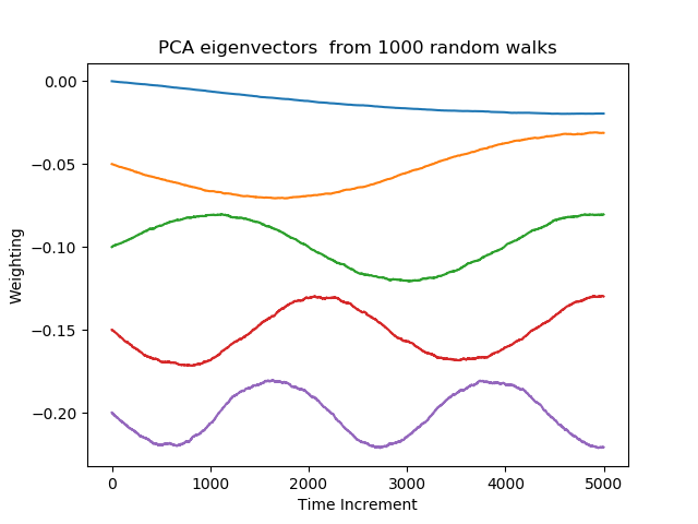
For completeness, I show the PCA eigenvectors from the series since I alluded to this in my comment. It shows that the variance in the dataset is composed of changes of different frequency.

So why does this happen?

The key is that the underlying data generating process consistently averages adding the mean step, so over long runs the variance due to accumulated mean steps will eventually overpower the variance in the individual steps and tend towards 1 (except for 0 mean). The rate at which this happens will depend on the relative size of the mean and the standard deviation of the underlying process.

Simulation Code

Here's python code should you wish to play around from sklearn.decomposition import PCA import numpy as np import matplotlib.pyplot as plt import scipy

# SETUP simulation parameters
N_intervals =  5000 # can restrict range to see how interval sample range affects behaviour
N_samples = 1000 
N_PCs = 5
fig_num = 0
mu = 1
sd = 1
np.random.seed(8736)

sim_data = np.empty((N_samples,N_intervals))
# starts the samples at zero, to start at random positions 
sim_data[:,0] = np.zeros((N_samples)) 

# simulate time dependent random walk - you can replace the step change with 
# any distribution or stochastic process you want. The -0.5 gives a mean change of 0
for i in range(1,N_intervals):
    sim_data[:,i] = sim_data[:,i-1] + np.random.normal( mu , sd , (N_samples) )

# plot how the data varies against time for each run
fig_num =+ 1
plt.figure(fig_num)
plt.plot(sim_data.T)
plt.xlabel('Time Increment')
plt.ylabel('Value')
title = str( N_samples ) + ' simulated random time walks' 
plt.title(title)
plt.figure(fig_num).savefig( title + '.png')

# plot dispersion against interval 
sim_data_sd = np.std(sim_data,axis=0)
fig_num += 1
plt.figure(fig_num)
plt.plot(sim_data_sd)
plt.xlabel('Time Increment')
plt.ylabel('SD')
title = ( 'Standard Devation between ' + str( N_samples ) + 
         ' simulated random time walks vs time interval' )
plt.title(title)
plt.figure(fig_num).savefig( title + '.png')

# plot R2 against interval 
ranges = (10**np.arange(np.log10(50),np.log10(5001),0.25)).astype('int')
r = np.empty((N_samples,np.shape(ranges)[0]))
for iSam in range(N_samples):
    for iInt in range(ranges.shape[0]):
        a , b , r[iSam,iInt], p , se = ( 
            scipy.stats.linregress(np.arange(ranges[iInt]), sim_data[iSam,:ranges[iInt]]) )
        #currently not storing slope a or intercept b as only looking at R
fig_num += 1
plt.figure(fig_num)
plt.plot(ranges, r.T**2,'.') # this is one version of R2
plt.xlabel('Time Increment')
plt.ylabel('$R^2$')
title = ( 'Individal R2 for ' + str( N_samples ) + 
         ' simulated random time walks vs interval' )
plt.title(title)
plt.figure(fig_num).savefig( title + '.png')

fig_num += 1
plt.figure(fig_num)
plt.plot(ranges, np.mean(r.T**2,axis=1),'.') # this is one version of R2
plt.xlabel('Time Increment')
plt.ylabel('$R^2$')
title = ( 'mean R2 for ' + str( N_samples ) + 
         ' simulated random time walks vs interval' )
plt.title(title)
plt.figure(fig_num).savefig( title + '.png')


# Here's the PCA eigenvectors
random_walk_PCA = PCA( n_components=N_PCs )  # fit a PCA to the simulated data
random_walk_PCA.fit(sim_data)
fig_num = fig_num+1
plt.figure(fig_num)
plt.plot(random_walk_PCA.components_.T + np.arange(0,-0.05*N_PCs,-0.05))
plt.xlabel('Time Increment')
plt.ylabel('Weighting')
title = 'PCA eigenvectors  from ' + str( N_samples ) + ' random walks' 
plt.title(title)
plt.figure(fig_num).savefig( title + '.png' )