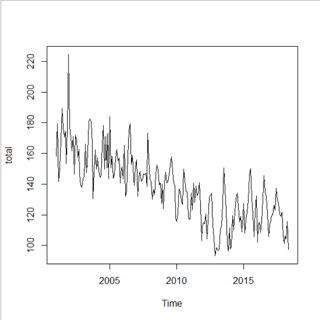
I have a ts that has the average monthly measure of pollutants in the air and i'm trying to use a SARIMA$(p,d,q)(P,D,Q)$ to model it but I'm having trouble determining the order because I'm somehow not able to remove the seasonality from the data.
So, because there's both trend and seasonality I took the 12th difference to account for the high yearly average in the summer months, and then plotted the decomposed series
m_diff1 = diff(m_ts, 12)
plot(m_diff1)

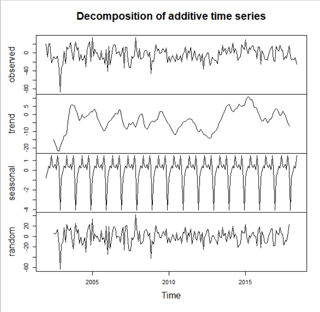
plot(decompose(m_diff1))
Which is weird to me because it got rid of the linear trend and not the seasonal trend? And when I decided to difference again (this time by 1) to "account" for the linear trend but I still wasn't able to remove the seasonality.
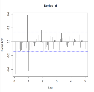
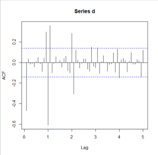
Nonetheless the PACF and ACF plots look like this:
 ,
,  Which I'm not sure they tell me much considering I wasn't able to successfully deal with the seasonality in the time series. Also, side-note I'm doing this all in R, here's some of the series:
    structure(c(158.149232493735, 179.540288982211, 141.55529618627,
    150.845437794367, 168.274600153682, 189.320502016778), .Dim = c(6L,
    1L), .Dimnames = list(NULL, "total"), .Tsp = c(2001, 2001.41666666667,
    12), class = "ts")
and I'm using this site: https://online.stat.psu.edu/stat510/lesson/4/4.1 as a guide
So, how can I properly deal with the seasonality and trend to eventually get the correct ACF/PACF so I can determine the order of the SARIMA model? TIA.
Edit: The .csv from which my time series is coming from:
structure(list(month = c(1, 2, 3, 4, 5, 6), year = c(2001, 2001,
2001, 2001, 2001, 2001), date = structure(c(11338, 11367.5, 11397,
11427.5, 11458, 11488.5), class = "Date"), BEN = c(4.28886198366742,
4.38743793320742, 3.11104641427313, 2.56016353321633, 2.70548122626857,
2.74478118843687), CO = c(1.15802566116617, 1.23165656956996,
0.833924652172606, 0.684889720572276, 0.773497978874483, 0.729142271395529
), EBE = c(3.93199632361959, 4.19389259556923, 2.96451683519944,
2.74148728405705, 3.01795589827371, 3.22289424876417), NMHC = c(0.238906290845672,
0.255622885192273, 0.173836570596142, 0.122209842180147, 0.154969322011947,
0.182527304410567), NO_2 = c(57.0312570252329, 64.6602424449942,
49.3705168821429, 53.0761352674492, 64.0999323771752, 67.647206830732
), O_3 = c(19.5139354574232, 20.5383038087111, 29.0497742674487,
40.2824860453053, 41.0452354173344, 46.1043441730726), PM10 = c(29.449900436516,
37.2815273458053, 24.9915362792256, 25.72564503371, 28.8485156121304,
39.3479598829578), SO_2 = c(24.97849825792, 29.0985261701844,
18.5026587019837, 15.1563261270824, 14.7196862860246, 15.2449743549489
), TCH = c(1.54189654517488, 1.54131730478954, 1.43556658648871,
1.34656043877617, 1.39043968735192, 1.39899987053764), TOL = c(16.0159545121689,
16.351761924188, 11.1219189967391, 9.14953450201853, 11.5188863482367,
12.6976718915217), station = c(28079021.6430525, 28079021.6153846,
28079022.2668467, 28079021.9261736, 28079021.8, 28079021.9223757
), day = c(16, 14.5, 16, 15.5, 16, 15.5), total = c(158.149232493735,
179.540288982211, 141.55529618627, 150.845437794367, 168.274600153682,
189.320502016778)), row.names = c(NA, -6L), groups = structure(list(
    month = c(1, 2, 3, 4, 5, 6), .rows = list(1L, 2L, 3L, 4L,
        5L, 6L)), row.names = c(NA, -6L), class = c("tbl_df",
"tbl", "data.frame"), .drop = TRUE), class = c("grouped_df",
"tbl_df", "tbl", "data.frame"))


