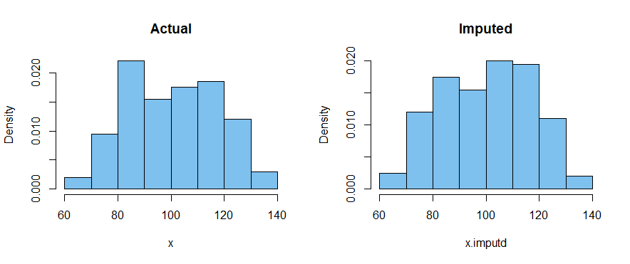
Example with normal data. Suppose the real data are a random sample of size $n=200$ from $\mathsf{Norm}(\mu=100, \sigma=15),$ but you don't know $\mu$ or $\sigma$ and seek to estimate them. In the example below I'd estimate $\mu$ by $\bar X = 100.21$ and $\sigma$ by $S = 14.5,$ Both estimates are pretty good. (Simulation and computations in R.)
set.seed(402)  # for reproducibility
x = rnorm(200, 100, 15)
mean(x);  sd(x)
# [1] 100.2051   # aprx 100
# [1] 14.5031    # aprx 15
Now suppose that 25% of these data are missing. (That's a large proportion, but I'm
trying to make a point.) If I replace the missing observations by the mean of the 150 non-missing observations, let's see what my estimates of $\mu$ and $\sigma$ would be.
x.nonmis = x[51:200]  # for simplicity suppose first 50 are missing
x.imputd = c( rep(mean(x.nonmis), 50),  x.nonmis )
length(x.imputd);  mean(x.imputd);  sd(x.imputd)
# [1] 200               # 'x.imputd' has proper length 200
# [1] 100.3445          # aprx 100
# [1] 12.58591          # much smaller than 15
Now we estimate $\mu$ as $\bar X_{imp} = 100.3,$ which is not a bad estimate, but potentially (as here) worse than the mean of the actual data. However, we now estimate $\sigma$ as $S_{imp} = 12.6,$ which is quite a bit below both the true $\sigma$ and its better estimate 14.5 from actual data.
Example with exponential data. If the data are strongly right-skewed (as for data from an exponential population), then replacing missing data with the mean of nonmissing data could mask the skewness so that we may be surprised that the data do not reflect how heavy the right tail of the population really is.
set.seed(2020)  # for reproducibility
x = rexp(200, .01)
mean(x);  sd(x)
# [1] 108.0259   # aprx 100
# [1] 110.1757   # aprx 100
x.nonmis = x[51:200]  # for simplicity suppose first 50 are missing
x.imputd = c( rep(mean(x.nonmis), 50),  x.nonmis )
length(x.imputd);  mean(x.imputd);  sd(x.imputd)
# [1] 200
# [1] 106.7967   # aprx 100
# [1] 89.21266   # smaller than 100
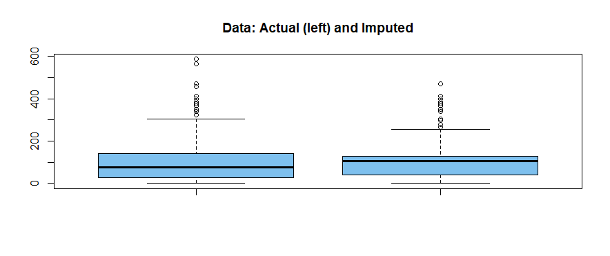
boxplot(x, x.imputd, col="skyblue2", main="Data: Actual (left) and Imputed")
The boxplot shows more skewness in the actual data (many observations in high tail)
than in the 'imputed' data.

Example with bimodal data. Again here, when we substitute missing values with
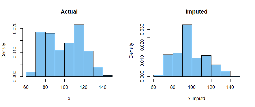
the mean of the nonmissing observations, the population standard deviation is underestimated. Perhaps more seriously, the large number of imputed values at the center of the 'imputed' sample masks the bimodal nature of the data.
set.seed(1234)  # for reproducibility
x1 = rnorm(100, 85, 10);  x2 = rnorm(100, 115, 10)
x  = sample(c(x1,x2))  # randomly scramble order
mean(x);  sd(x)
# [1] 99.42241
# [1] 18.97779
x.nonmis = x[51:200]  # for simplicity suppose first 50 are missing
x.imputd = c( rep(mean(x.nonmis), 50),  x.nonmis )
length(x.imputd);  mean(x.imputd);  sd(x.imputd)
# [1] 200
# [1] 99.16315
# [1] 16.41451
par(mfrow=c(1,2))
 hist(x,        prob=T, col="skyblue2", main="Actual")
 hist(x.imputd, prob=T, col="skyblue2", main="Imputed")
par(mfrow=c(1,1))

In general: Replacing missing data by the mean of nonmissing data causes the population SD to be underestimated, but may also obscure important
features of the population from which the data were sampled.
Note: As @benso8 observes, using the mean of nonmissing data to replace missing observations is not always a bad idea. As mentioned in the Question, this method does reduce the variability. There will necessarily be drawbacks to any scheme
for dealing with missing data. The Question asked for speculation about possible disadvantages other than variance reduction for this method. I tried to illustrate a couple of possibilities in my last two examples.
Tentative alternative method: I am no expert in data mining. So I very tentatively propose an alternative method. I don't claim it's a new idea.
Instead of replacing all $m$ missing items with the sample mean of the nonmissing ones, one might take a random sample of size $m$ from among the nonmissing observations, and scale it so that the $m$ items have the same mean and SD as the nonmissing data. Then combine the rescaled $m$ items with the nonmissing ones to get an 'imputed' sample with nearly the same mean and SD as the nonmissing part of the sample.
The result should not systematically underestimate the population SD, and may better preserve features of the population such as skewness and bimodality. (Comments welcome.)
This idea is explored for bimodal data below:
set.seed(4321)  # for reproducibility
x1 = rnorm(100, 85, 10);  x2 = rnorm(100, 115, 10)
x  = sample(c(x1,x2))  # scrmble
mean(x);  sd(x)
# [1] 100.5299
# [1] 17.03368
x.nonmis = x[51:200]  # for simplicity suppose first 50 are missing
an       = mean(x.nonmis);  sn = sd(x.nonmis)
x.subt   = sample(x.nonmis, 50)      # temporary unscaled substitutes
as       = mean(x.subt); ss = sd(x.subt)
x.sub    = ((x.subt - as)/ss)*sn + an # scaled substitutes

x.imputd = c( x.sub,  x.nonmis )
mean(x.imputd);  sd(x.imputd)
# [1] 100.0694    # aprx same as mean of nonmissing
# [1] 16.83213    # aprx same os SD of nonmissing

par(mfrow=c(1,2))
 hist(x,        prob=T, col="skyblue2", main="Actual")
 hist(x.imputd, prob=T, col="skyblue2", main="Imputed")
par(mfrow=c(1,1))
