How do you compare linear model vs non-linear (nls) model in R?

Question

I am trying to model some data, and as part of the modeling, I tried using a linear model (using the lm function) and a non-linear model (using the nls) function.

• Model 1: a linear model which has degrees of freedom (df), (AIC) = 2, 2130

• Model 2: a non-linear model which has df, AIC= 4, 2128.

• Model 3: I took model 2 above and fixed a parameter to the estimated value in model 2. It resulted in df, AIC= 3, 2126.

My question is: how to select the best fitting model from the above candidate models? Can I simply use AIC (lower is better) and therefore select model 3?

Answer 1

Caveat-Infused Answer

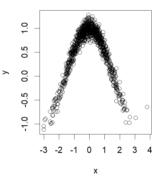
Some of the others here are correct in stating that you can use AIC/BIC criterion for deciding between models, but I want to stress that it isn't the only thing to consider. I highlight a simulated example in R. Here I have made curvilinear data:

#### Load Libraries and Theme ####
library(tidyverse)
library(mgcv)
library(ggpubr)
theme_set(theme_bw())

#### Simulate Curvilinear Data ####
set.seed(1)
x <- rnorm(n=1000)
y <- cos(x) + rnorm(n=1000,sd=.1)
plot(x,y)
df <- data.frame(x,y)

Shown below:

Fitting Models

Since the data appears fairly curvilinear, I have fit two opposing models: one that just uses an exponential term in lm, and the other which uses a spline in a generalized additive model using gam in the mgcv package.

#### Fit Exponent Only Model ####
fit.1 <- lm(y ~ x + I(x^2))

#### Fit Spline Model ####
fit.2 <- gam(y ~ s(x),
             method = "REML")

Below are the output from summary(fit.1) and summary(fit.2):

> summary(fit.1)

Call:
lm(formula = y ~ x + I(x^2))

Residuals:
     Min       1Q   Median       3Q      Max 
-0.50225 -0.10252  0.00233  0.09559  2.72887 

Coefficients:
             Estimate Std. Error t value Pr(>|t|)    
(Intercept)  0.900580   0.006674 134.931   <2e-16 ***
x            0.002338   0.005270   0.444    0.657    
I(x^2)      -0.295418   0.003603 -81.993   <2e-16 ***
---
Signif. codes:  0 ‘***’ 0.001 ‘**’ 0.01 ‘*’ 0.05 ‘.’ 0.1 ‘ ’ 1

Residual standard error: 0.1723 on 997 degrees of freedom
Multiple R-squared:  0.871, Adjusted R-squared:  0.8707 
F-statistic:  3366 on 2 and 997 DF,  p-value: < 2.2e-16

> summary(fit.2)

Family: gaussian 
Link function: identity 

Formula:
y ~ s(x)

Parametric coefficients:
            Estimate Std. Error t value Pr(>|t|)    
(Intercept)   0.5844     0.0033   177.1   <2e-16 ***
---
Signif. codes:  0 ‘***’ 0.001 ‘**’ 0.01 ‘*’ 0.05 ‘.’ 0.1 ‘ ’ 1

Approximate significance of smooth terms:
       edf Ref.df    F p-value    
s(x) 8.818  8.991 2233  <2e-16 ***
---
Signif. codes:  0 ‘***’ 0.001 ‘**’ 0.01 ‘*’ 0.05 ‘.’ 0.1 ‘ ’ 1

R-sq.(adj) =  0.953   Deviance explained = 95.3%
-REML = -812.91  Scale est. = 0.010888  n = 1000

We can already see that the spline regression has a higher $R^2$ value than the quadratic polynomial model. So we would expect to at least some degree that it performs better in general.

AIC/BIC

If we look at the AIC/BIC of the models as prescribed:

#### Print AIC/BIC of Models ####
cat("----------------------",
    "\nModel AIC/BIC",
    "\n----------------------",
    "\nModel 1 AIC:",
    AIC(fit.1),
    "\nModel 1 BIC:",
    BIC(fit.1),
    "\n----------------------",
    "\nModel 2 AIC:",
    AIC(fit.2),
    "\nModel 2 BIC:",
    BIC(fit.2),
    "\n----------------------")

You will find that the gam fit is substantially lower for both criterion:

---------------------- 
Model AIC/BIC 
---------------------- 
Model 1 AIC: -674.0088 
Model 1 BIC: -654.3778 
---------------------- 
Model 2 AIC: -1670.372 
Model 2 BIC: -1617.155 
----------------------

Do we throw out the first model? Let's check the plots first.

Plotting

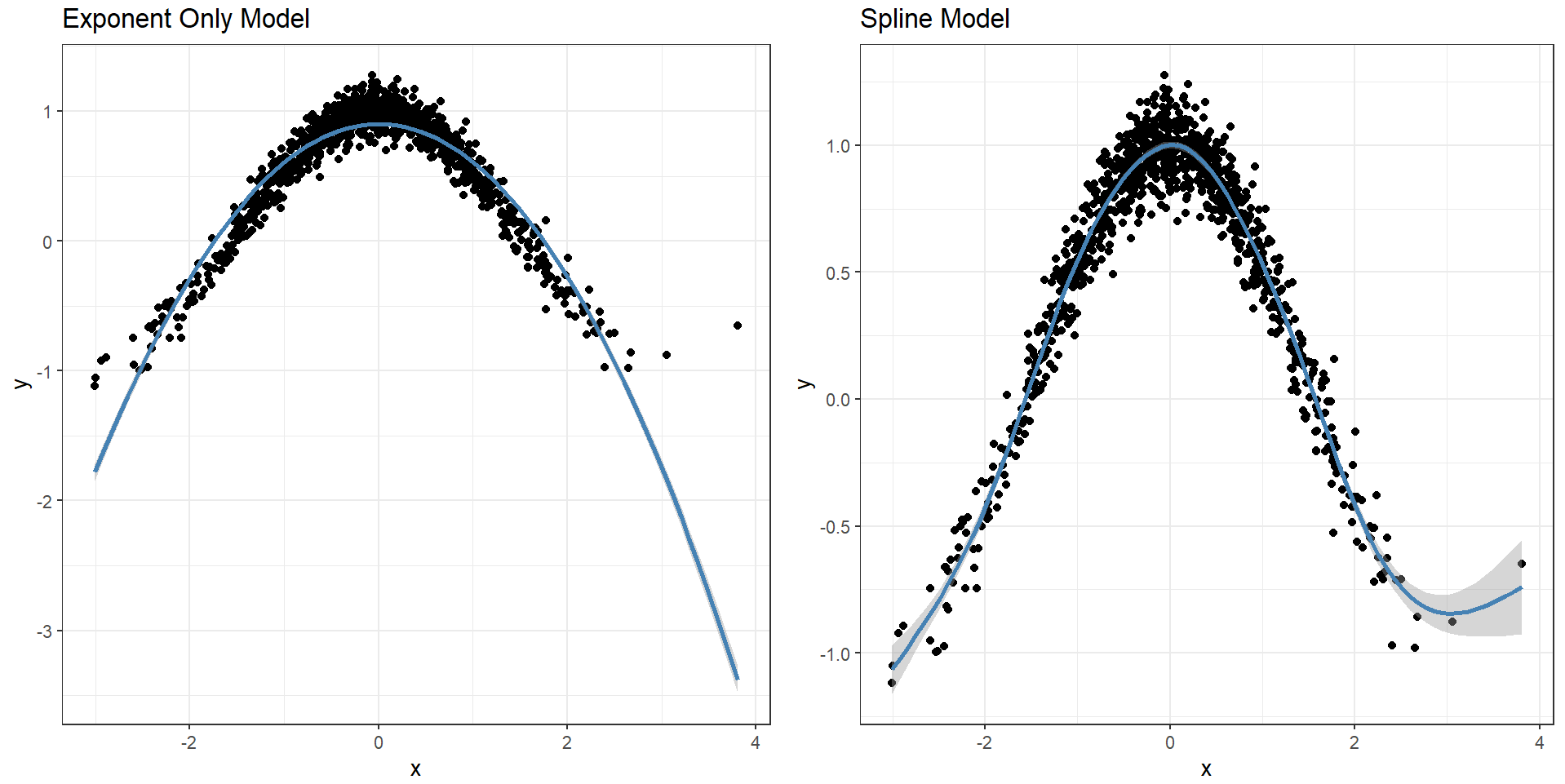
To make sure we are getting what we asked for, we can plot both of the models directly with ggplot. I have also arranged them into one window with ggarrange.

#### Plot Models ####
p1 <- df %>% 
  ggplot(aes(x,y))+
  geom_point()+
  geom_smooth(
    method = "lm",
    formula = y ~ x + I(x^2),
    color = "steelblue"
  )+
  labs(title = "Exponent Only Model")

p2 <- df %>% 
  ggplot(aes(x,y))+
  geom_point()+
  geom_smooth(
    method = "gam",
    formula = y ~ s(x),
    color = "steelblue"
  )+
  labs(title = "Spline Model")

ggarrange(p1,p2)

Shown below:

You can see both have mapped a curvilinear trend, and it's quite obvious they would fit/predict better than a simple first-order polynomial trend ("linear"). However, you can see why the first model's $R^2$ was lower...it has overfit a global shape to the data and totally misses the uptick in data near the upper range to the right. Assuming we want to use this to infer the relationship outside of a laboratory, our predictions would be completely off regardless of any AIC/BIC criterion. We can see this if we check the residuals...

Residual Inspection

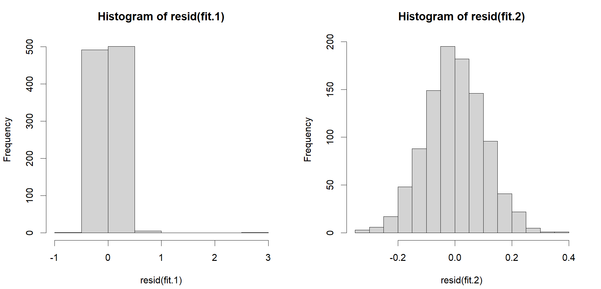
A quick look at the residuals will show that the AIC/BIC has done nothing to answer a much larger issue...the sheer volume of error in the first model. See the residual plots below as an example.

#### Check Residuals ####
par(mfrow=c(1,2))
hist(resid(fit.1))
hist(resid(fit.2))

We can see the residuals look quite normal in the second plot for the better performing GAM, but the residuals are bizarrely smooshed into two bins. Clearly the GAM model is more accurate.

Conclusion

In summation, the AIC/BIC criterion are useful tools, but like all things in regression, you should make sure you are looking at the whole picture first.

Answer 2

The question is indeed rather theoretical. What is the best theoretical model by construction (i.e. how do the variables connect to each other? Is the theoretical dependence of linear or non-linear nature?).

However, if that is not possible, I suggest to compare the models using BIC and AIC as well and select some model inbetween those two. From my personal experience AIC is better for predictions and BIC better for fitting (explanatory).

Answer 3

You will find unending debates on the question. There is no good answer on that question. Generally, people tend to prefer BIC rather than AIC. BIC selects more parcimonious models because the penalty for the number of parameters is higher.

If you are more interested in predictions, you might use other performance criterion. Especially root mean square error (RMSE).

I think you will find many interesting debates on this question on CrossValidated.

Answer 4

If you are interested in predictions: The MAPE function in R, or mean absolute percentage error (MAPE), is a measure of prediction accuracy of a forecasting method in statistics.

install.packages("MLmetrics") 
library(MLmetrics)
MAPE(predict(model),real_values)