I am trying to see if there is a relation between the proportion of target vs non target species in some communities and their phylogenetic structure. I cannot show you the real data but it looks something similar to this (although I have over 18000 data points and 'hab' has 12 levels):
df <- structure(list(hab = structure(c(6L, 6L, 6L, 6L, 6L, 6L, 6L,12L, 12L, 9L),
   .Label = c("Eur_nitro_herb", "Forest_deciduous","Forest_everg_Eur",
   "Forest_med", "Grass_alp", "Grass_mont_subalp","Margin_mantle", "Med_nitro_herb", "Rocks",     "Shrub_med", "Shrub_mont_subalp","Wet_humid"), class = "factor"),
   ses_mpd = c(0.05408747785078,-0.578266990137644, -1.48812316684822, -0.345401572814568,  0.124151290090708,-1.51817069020564, 0.0530607986221243, 0.00261416940904258, 0.665908557766837,-0.701477005797007),
   target = c(1, 2, 3, 1, 2, 0, 0, 0, 0, 1),non_target = c(32, 27, 20, 30, 34, 26, 30, 9, 12, 6)), row.names = c(1L,2L, 3L, 4L, 5L, 6L, 7L, 18793L, 18794L, 18795L), class = "data.frame")

df
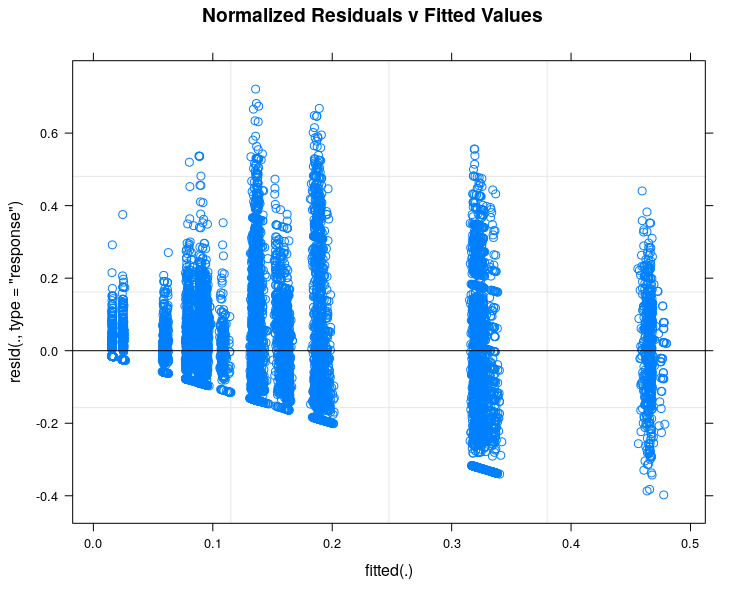
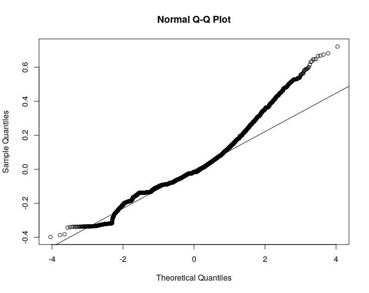
ses.mpd as calculated by the picante package is a standarized size effect so it can take positive and negative values as well as zero. I want to see the relationship between proportion of target and non target with ses_mpd controlling for possible differences between habitats. I have used a Generalized Linear Mixed Model to do so but when I check the residuals they look fairly skewed:
library(lme4)
mod<-glmer(cbind(target,non_target)~ses_mpd+(1|hab), family = binomial(logit), data = df)
plot(mod, resid(., type='response')~fitted(.), main="Normalized Residuals v Fitted Values",abline=c(0,0))
res <- resid(mod, type="response")
qqnorm(res)
qqline(res)
Given the large sample size I was expecting that the residuals would be normal but I was clearly wrong. I guess that these results cannot be trusted so my question is if there is any other way to analyzed this data.
Cheers and thanks in advance.


