How many observations are needed for correlations to be statistically sound?

Question

I have a group of 450 high-value soccer players. I'm trying to find common changes in skill metrics in this group of players to see their effects on the players' valuations and reputations by using a Pearson correlation.

But skills are dependent on the player's position. So when I divide the group further, I get groups of 60-115 players/observations per group, which the exception of goalkeepers, whose group total is about 15.

After doing some research, I can't seem to find a source for a minimum number of observations that allow correlations to stabilize. Some say it's as low as n=20, where as another study conducted for psychological applications put the number at 250 before correlations to stabilize. I even encountered this question here, but it only really refers to standard error in relation to standard correlation with low n as the solution, but not really what is considered a standard for statistical significance.

Since I'm examining a certain type of player, where said correlations could help pick out future elite players, would the 450 be considered their own population so the n doesn't matter as much since it represents the population?

Basically, do the number of observations I have for each group (except the goalkeepers) enough to calculate generally stable correlation coefficients?

Answer 1

The sample size required depends on the particular situation. The usual significance test is for the null hypothesis that $\rho = 0.$ So if your situation has $\rho$ far from $0,$ it will be easier to reject $H_0.$

Below I simulate $n = 15$ pairs in a model with $\rho = 0.95.$ Results from 100,000 samples following this model are that $H_0: \rho = 0$ is almost always rejected (power of the test about $0.98).$ So in at least some such situations $n = 15$ is plenty.

set.seed(2020)
rho = .85; n = 15
m = 10^5;  pv = r = numeric(m)
for (i in 1:m) {
 x = rnorm(n); z = rnorm(n)
 y = x*rho + z*sqrt(1-rho^2)
 r[i] = cor(x,y)
 pv[i] = cor.test(x,y)$p.val
}
summary(r)
     Min. 1st Qu.  Median    Mean 3rd Qu.    Max. 
  -0.1691  0.8005  0.8589  0.8402  0.9011  0.9893 
mean(pv < 0.05)
[1] 0.9933  # power of test

It is easy to change $n$ and $\rho$ in the simulation above to explore other situations.

For example, with $n = 15, \rho = .75,$ the power is about $0.94.$ Also, with $n = 15, \rho = 0.65,$ I get power only about $0.79,$ but for $\rho = 0.65$ increasing the sample size to $n = 25$ raises the power to about $0.96.$ If you can give more of the particulars of your situation, maybe one of us will give an answer that matches your situation more closely.

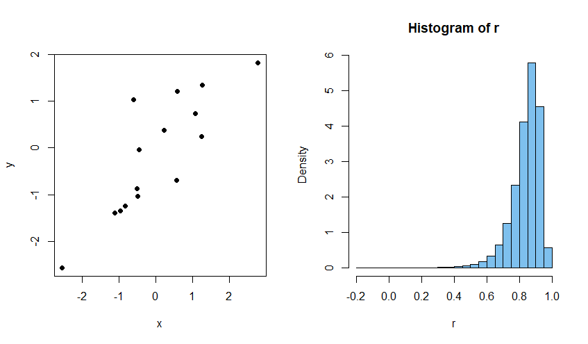
The figure at the left below shows a plot of the fifteen $(x,y)$ pairs in the first of the 100,000 samples of the main simulation ($\rho = 0.85.)$ Its sample correlation is $r = 0.788$ and $H_0$ rejected. At the right is a histogram of the sample correlations $r$ for all of the samples.

Note: The test for $H_0: \rho=0$ against $H_0: \rho \ne 0$ in all of the computations above (using cor.test) assumes that the $X$ and $Y$ are jointly normally distributed.

Answer 2

This addresses part of the question:

Since I'm examining a certain type of player, where said correlations could help pick out future elite players, would the 450 be considered their own population[?]

This isn't a solution as it is not even logically consistent.

1. You're intending or hoping that present players are a sample of a population of possible "high-value" players, however you word it. Or that the target population is all possible players (with extra criteria, too), but necessarily the sampled population is present players (noting precise extra criteria, and that we need data from their pasts to have data at all). The distinction between target population and sampled population is sometimes helpful. The population is not defined very precisely in your question. You presumably have some threshold in terms of standard of player and perhaps other criteria too.

2. Other way round, if present players are a population, inference is not relevant at all except if you are imagining measurement error as a problem, unlikely for your example. The question of whether the population is large enough isn't meaningless, but it is hard to give it a precise meaning. You could compare other populations, for example, but then you're back to thinking of them as being other samples in some sense.