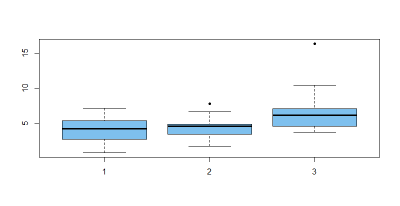
Example using data simulated in R.
set.seed(1234)
x1 = rgamma(15, 3, .6)
x2 = rgamma(15, 3, .6) + .5
x3 = rgamma(15, 3, .6) + 2
x = c(x1,x2,x3);  g = rep(1:3, each=15)
In R, the K-W test output does not mention $H_0,$ which is rejected
for my example, with P-value 0.025. You can use two-sample Wilcoxon
tests to see which pairs of medians differ significantly.
kruskal.test(x ~ g)

        Kruskal-Wallis rank sum test

data:  x by g
 Kruskal-Wallis chi-squared = 7.4025, df = 2, p-value = 0.02469
Boxplots show sample medians:
boxplot(x ~ g, col="skyblue2", pch=20)

From the simulation, we know that the population medians are $\eta_1 = 4.457, \eta_2 = 4.857, \eta_3 = 6.457.$
qgamma(.5, 3, .6)
[1] 4.456767
here are the sample medians:
median(x1);  median(x2);  median(x3)
[1] 4.215075
[1] 4.568092
[1] 6.14665
According to a 2-sample Wilcoxon test, the sample medians $H_1$ and $H_3$ differ significantly. If you do several such ad hoc tests you need to use some method to help avoid false discovery (such as Bonferroni).
wilcox.test(x1, x2)$p.val
[1] 0.6235943
wilcox.test(x1, x3)$p.val
[1] 0.01855373

