If $X \sim \mathsf{Norm}(\mu=0,\sigma=2)$ and
$Y \sim \mathsf{Norm}(\mu=0,\sigma=\sqrt{5}),$
then $Z = X+Y \sim
\mathsf{Norm}(\mu=0,\sigma=\sqrt{4+5} = 3).$
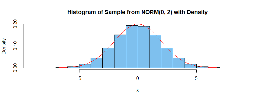
If you simulate many values of $X,$ then the a histogram
of those values imitates the density function of $\mathsf{Norm}(\mu=0,\sigma=2).$
Also, the sample mean of the many values $X_i$ will
be $\bar X \approx 0$ and the their standard
deviation will be $S_X = \frac{1}{n-1}\sum_{i=1}^n (X_i - \bar X)^2 \approx 2.$
Using R for the
simulating, summarizing, and graphing, we have:
set.seed(2020)
x = rnorm(10^5, 0, 2
summary(x); sd(x)
     Min.   1st Qu.    Median      Mean   3rd Qu.      Max.
-8.359695 -1.349914 -0.014586 -0.005547  1.339879  8.318011
[1] 1.994003  # aprx sigma.x = 2

hist(x, prob=T, col="skyblue2",
     main="Histogram of Sample from NORM(0, 2) with Density")
curve(dnorm(x, 0, 2), add=T, col="red")
Similarly, for $Y,$ but without the graph, we get:
summary(y); sd(y)
     Min.   1st Qu.    Median      Mean   3rd Qu.      Max.
-9.607853 -1.505329 -0.006414  0.001022  1.500837 10.620498
[1] 2.235846  # aprx sigma.y = sqrt(5) = 2.236
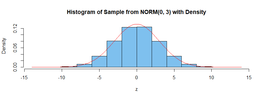
Finally, if you add simulated vectors of values x and y, you will simulate the distribution of
$$Z = X+Y \sim
\mathsf{Norm}(\mu=0,\sigma=\sqrt{4+5} = 3),$$
Thus, a data summary of z will show $\bar Z \approx 0$ and $S_Y \approx 3.$
z = x + y
summary(z);  sd(z)
      Min.    1st Qu.     Median       Mean    3rd Qu.       Max.
-13.299918  -2.027446  -0.003853  -0.004525   2.010361  12.703835
[1] 2.994405  # aprx sigma.z = 3

hist(z, prob=T, col="skyblue2",  ylim=c(0,.13),
     main="Histogram of Sample from NORM(0, 3) with Density")
curve(dnorm(x, 0, 3), add=T, col="red")
Notes: In case you are interested in details of R, here are a few.
(1) Normal probability functions in R, (such as rnorm to simulate and density dnorm, use the standard deviation $\sigma$ instead of the variance $\sigma^2.$
(2) If you are going to superimpose a density function on a histogram, then the histogram needs to be a 'density histogram'. This requires parameter prob=T in hist.
(3) The R procedure curve to plot a function requires the argument of the function always to be written as x--- regardless of the context.
(4) The parameter ylim=c(0,.13) of the procedure hist makes the plotting window tall enough to
accommodate the density curve without cutting off
its mode.
(5) When you write x + y in R for two vectors of the same length (here length $10^5 = 100,000)$ then R takes the
element-wise sum, yielding a vector of the same length.
The table below shows the first six out of 100,000 such additions.
head(cbind(x, y, z))
              x          y          z
[1,]  0.7539442  1.0037551  1.7576993
[2,]  0.6030967  0.2978469  0.9009436
[3,] -2.1960463  3.9858896  1.7898433
[4,] -2.2608118 -3.0263022 -5.2871140
[5,] -5.5930686  3.8786439 -1.7144247
[6,]  1.4411470  0.3790924  1.8202394

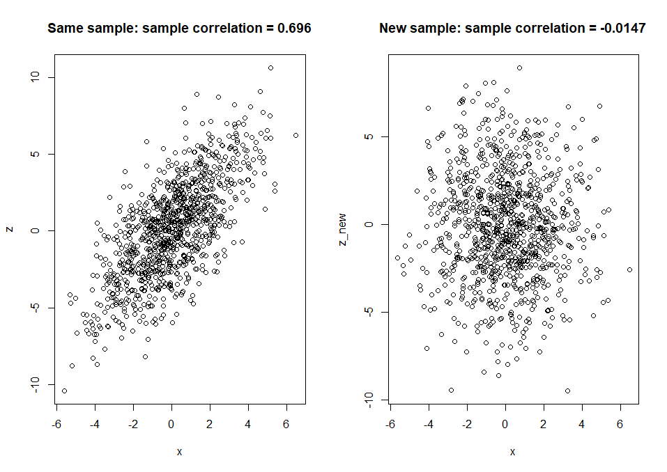


X, one forY, one forZ. As a guess, you probably don't want the samples to be independent, but how could we actually know that? You never said what you were trying to do. $\endgroup$