For 2-sample t tests. For two-sample t tests, I think it is now standard practice
to use the Welch two-sample t test, unless there is strong
prior evidence (say, from data of the same type) that population
variances are equal. In some statistical software packages the
Welch test is the default 2-sample t test, so that one must
specifically request the pooled version of the test if desired.
(For example, I know that the Welch test is the default in
both R and Minitab. I believe some other statistical software
programs show P-values for both tests.)
The Welch two-sample t test uses the
Satterthwaite DF, which is often smaller than the DF $n_1 + n_2 - 2$ of the pooled 2-sample t test (never larger). This means that the power of the Welch 2-sample t test is somewhat smaller than the power of the pooled test, often not enough smaller to matter for practical purposes. But some statisticians do make an exception to standard practice when sample sizes are very small and sample standard deviations are similar.
For one-way ANOVA. However, the Satterthwaite (or Welch) ANOVA, implemented in R as oneway.test, is relatively new, and there has not been the same level of scrutiny of the Satterthwaite ANOVA as there has been of the Satterthwaite 2-sample t test. A couple of limited simulation studies I have seen and my own experience have made me feel comfortable using the Satterthwaite ANOVA by default. But I don't think one can say yet that it is 'standard practice' to use the Satterthwaite ANOVA.
At this point, I would have to admit that strong preference for
the Satterthwaite one-way ANOVA is still a matter of personal opinion (even if fairly widespread). So we may see other answers here voicing different opinions.
Addendum: In response to a Comment, here is an example of simulation investigating
the behavior of the Welch ANOVA.
The two-sample pooled t test is known to behave badly
if sample sizes differ and the population from which the smaller sample was chosen has a larger variance than the other population. Specifically, if population means are the same, the true significance level can be inflated considerably.
Here we use simulation to investigate the behavior of a standard ANOVA (assuming equal population variances) in an analogous situation and compare the behavior the behavior of the Welch ANOVA in the same situation. In particular, we use sample sizes 5, 10, and 15, and respective population SDs
7, 3, and 1.
To make sure we assess precisely the versions of ANOVA implemented in R, we simulate 100,000 datasets, run both ANOVAs in R, and look at the 200,000 resulting P-vales.
Because R formats each ANOVA, only for us to use the P-value in each case, the code is inefficient and runs slowly.
set.seed(2020)
m = 10^5;  pv.e = pv.w = numeric(m)
for(i in 1:m){
 x1 = rnorm( 5, 50, 7)
 x2 = rnorm(10, 50, 3)
 x3 = rnorm(15, 50, 1)
 x = c(x1,x2,x3)
 g = as.factor(rep(1:3, c(5,10,15)))
 pv.w[i] = oneway.test(x~g)$p.val
 pv.e[i] = summary(aov(x~g))[[1]][1,5]
}
mean(pv.e <= .05)
[1] 0.2496
mean(pv.w <= .05)
[1] 0.05673
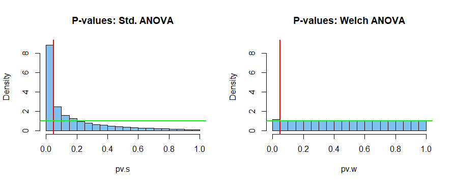
Quite wrongly assuming equal population variances, the standard ANOVA has an actual rejection rate of about 25%
for a test intended to be at the 5% level. This could
lead to massive false 'discovery' of population differences, where there are none.
By contrast, the Welch ANOVA has a rejection rate of
about 5.7% where the 5% level is intended. Not a perfect
result in this problematic situation, but a great improvement over the catastrophic result of the standard ANOVA.
Below are histograms of simulated P-values for the two tests.
Under the null hypothesis, the P-value of a test with a continuous test statistic should be standard uniform (with bars roughly the height of the green line).


