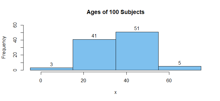
Suppose we have data as shown in the histogram below.
(Of course there are no ages below $0,$ but I wanted the
histogram bars to be of equal widths.)

Suppose we make the simplifying approximation that all ages
in each of the $k = 4$ histogram bins are at the centers of their intervals.
Then we get frequencies $3, 41, 51, 5$ (for $n = 100$ subjects altogether) 'located' at midpoints
$7, 25, 45, 65.$
Then the sample mean can be estimated as
$$\bar X \approx \frac{1}{n}\sum_{i = 1}^k f_im_i = 36.66.$$
The average was computed, using R statistical software as
a calculator, as follows:
f = c(3, 41, 51, 5)
m = c(7, 25, 45, 65)
a = sum(f*m)/100;  a
[1] 36.66
Perhaps somewhat less accurately, we can approximate the sample variance
as follows:
$$S^2 \approx \frac{1}{n-1}\sum_{i=1}^k f_i(m_i - \bar X)^2 = 159.358.$$
v = sum(f*(m-a)^2)/99;  v
[1] 159.358
Unless you have the original data, you can't know how accurately
$\bar X$ and $S^2$ are actually estimated by these formulas.
However, I simulated the heights in R, so we can check the
true values. For my simulated data the approximate values
happen to be quite accurate. [I suspect results in this
example turned out to be a little better than usual--especially because we used only four intervals.]
set.seed(2020)  # for reproducibility
x = round(rnorm(100, 35, 10))
summary(x)
   Min. 1st Qu.  Median    Mean 3rd Qu.    Max.
   5.00   29.00   36.00   36.09   42.25   67.00
var(x)
[1] 124.4666
Note: (1) Some years ago when computation was more tedious than it is with modern software, it was common practice to use the formulas shown here to approximate $\bar X$ and $S^2$ for large samples. Results are usually pretty good if you use a dozen or so intervals.
(2) Some elementary statistics books (especially high-school
AP statistics books) have formulas for estimating sample medians, other sample quantiles, estimating population modes from data summarized in the form of intervals and frequencies.
(3) See this related Q&A.

