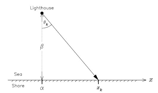
Interesting problem indeed. Three non-Bayesian solutions follow.
Classical Physicist's view
Here's my physicist's solution to it.
$$\alpha=median[x_k]=F^{-1}(1/2)$$
$$\beta=F^{-1}(3/4)-F^{-1}(1/4)$$
Here $F$ is the empirical CDF of Cauchy distribution, or you could also call it a quantile (percentile) function.

Cauchy distribution (aka Breit-Wigner in physics) has no mean, but it is symmetric. So, the median is a decent estimate of the $\alpha$.
Since, it has no variance either, in physics when using this distribution the notion of width at half height is used to describe its dispersion. It happens so that the width at half height of PDF is $\beta$ and corresponds to the span between first and third quartiles (interquartile range).
MLE
Maximum likelihood estimation, of course, is more efficient. However, mine is very simple and intuitive.
OLS (doesn't work)
There's also a terrible regression solution. Look at the quantile function of the distribution:
$$Q(p; \alpha,\beta) = \alpha + \beta\,\tan\left[\pi\left(p-\tfrac{1}{2}\right)\right]$$
It appears that, we can convert it into OLS problem (assuming $x_k$ are ordered!):
$$x_k = \alpha + \beta\,\tan\left[\pi\left((k-1/2)/N-\tfrac{1}{2}\right)\right]$$
$$x_k = \alpha + \beta\,z_k,$$
where $z_k=\tan\left[\pi\left((k-1/2)/N-\tfrac{1}{2}\right)\right]$
OLS will give you immediately the estimates $\hat\alpha,\hat\beta$.
The problem is that, OLS assumes finite variance, and we don't have it with Cauchy. So, the output of OLS is garbage. Here's R code to experiment and see how my first method is pretty robust.
alpha <- 10 # unkonwn true values
beta  <- 30 # this is known for now
##################
set.seed(123)
N       <- 1024
theta_k <- runif(N,-pi/2,pi/2)
x_k     <- beta * tan(theta_k) + alpha
q123 = quantile(x_k,c(1/4,1/2,3/4),type=1)
print("alpha")
print(q123[2])
print("beta")
print((q123[3] - q123[1])/2)

y = sort(x_k)
x = tan(pi*((seq(1:N)-0.5)/N-1/2))
fit = lm(y~x)
print(fit)
Outputs:
alpha <- 10 # unkonwn true values
beta  <- 30 # this is known for now
##################
set.seed(123)
N       <- 1024
theta_k <- runif(N,-pi/2,pi/2)
x_k     <- beta * tan(theta_k) + alpha
q123 = quantile(x_k,c(1/4,1/2,3/4),type=1)
print("alpha")
print(q123[2])
print("beta")
print((q123[3] - q123[1])/2)

y = sort(x_k)
x = tan(pi*((seq(1:N)-0.5)/N-1/2))
fit = lm(y~x)
print(fit)

