3
$\begingroup$

I think this question may be better split into univariate regression and multiple regression using OLS. Here we assume $\hat{\beta}_i$ are the "slopes", where $i > 0$, and $\hat{\beta}_0$ is the intercept.


For univariate regression, if you performed OLS, and obtained $\hat{\beta}_1 = 0$ (slope), then this means the line of best fit determined by OLS is a horizontal line located at some $\hat{\beta}_0$ offset from the horizontal axis. This also means the correlation coefficient between the regressor and response is zero, indicating no linear independence.

My question regarding this univariate case is, beyond linear independence, does the zero slope and zero correlation also indicate no monotonic relationship? If the data was monotonically increasing or decreasing, then there is no way the slope could end up zero?

A slope of zero does not rule out non-monotonic relationships. For example, consider $$ y = \sin(x) + \text{constant} $$. If the regressor is distributed from $x \in [0, n\pi]$, where $n$ is some even number, then OLS will give you $\hat{\beta_1} = 0$


For multiple regression, what are some obvious and subtle characteristics of $\hat{\beta}_i = 0$? Does it still indicate that there's no linear relationship between the i-th regressor and the response? Does it say anything about the $j$-th regressor, where $j \neq i$?

$\endgroup$

2 Answers 2

2
$\begingroup$

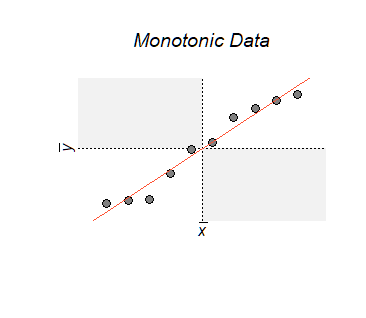
In the scatterplot of any $(x,y)$ data, the least squares fit (red line in the figure) will pass through the point of averages $(\bar x,\bar y),$ located at the intersection of the dotted axes.
enter image description here

When the relationship is monotonic, all the points lie in the unshaded quadrants. This means that to the left of the point of averages all the $x_i$ are less than $\bar x$ and monotonicity implies all the $y_i-\bar y$ in that region have the same sign. To the right of the point of averages all the $x_i-\bar x$ are positive but the signs of all the $y_i-\bar y$ are the opposite of what they were to the left. Unless these data lie on a vertical or horizontal line, at least one of the products $(x_i-\bar x)(y_i-\bar y)$ is nonzero. Consequently,

When the relationship between $x$ and $y$ is monotonic, the sum of the $(x_i-\bar x)(y_i-\bar y)$ is nonzero: positive when the relationship is a positive one, negative when the relationship is a negative one.

The least-squares slope, being a positive multiple of this sum, therefore is nonzero. The special cases of points along a horizontal line correspond to zero correlation and points along a vertical line correspond to undefined correlation (and undefined least-squares fit), so they are no exceptions to this general conclusion.

The converse of this implication is logically equivalent to it:

When the least-squares slope is zero, the relationship cannot be monotonic (unless the y-values are constant).


For multiple regression with a fit $\hat y = \hat \beta x + \hat \beta_2 x_2 + \cdots \hat \beta_p x_p,$ the coefficient $\hat \beta$ depends on the other variables included in the regression, as described at https://stats.stackexchange.com/a/46508/919. That is, you regress $y$ and $x$ separately against all the other variables and work with their residuals. This is perhaps the simplest way to understand what $\hat \beta=0$ means:

$\hat \beta=0$ implies that after taking out the effects of all other variables, replacing $x$ and $y$ by their residuals $x^\prime$ and $y^\prime$ respectively, then either $y^\prime$ is constant or there is no monotonic relationship between $x^\prime$ and $y^\prime.$


References

If you didn't know the OLS line passes through the point of averages or that the OLS (univariate) slope is proportional to the paired products of the $x$ and $y$ residuals, then please read the introductory section about correlation and regression in Freedman, Pisani, & Purves Statistics (any edition). Older editions are inexpensive and widely available.

My characterization of multiple regression as a univariate regression of the residuals is a core idea in Mosteller, Frederick, John Tukey. 1977. Data Analysis and Regression: A Second Course in Statistics. 1st edition.

$\endgroup$
-1
$\begingroup$

For the multivariate case, it would mean that there is no significant relationship between that particular predictor and the dependant variable

$\endgroup$
3
  • $\begingroup$ Say $\hat{\beta}_1 = 0$, and you have some $X_2$ that is correlated with $X_1$. If you removed $X_2$, the $\hat{\beta}_1$ could then be non-zero? $\endgroup$ Commented Jul 7, 2020 at 22:33
  • 3
    $\begingroup$ This answer is phrased in a way that many readers might misunderstand, because "no significant relationship" (a) doesn't answer any part of the question and (b) has a meaning only in the context of the other explanatory variables. The importance of this is manifest in a situation where $X_1=Y$ and $X_2$ differs only slightly from $Y:$ the univariate regression of $Y$ on $X_2$ can exhibit a strong, significant, linear relationship while the coefficient estimate of $X_2$ in the bivariate regression of $Y$ on $(X_1,X_2)$ may be zero. $\endgroup$
    – whuber
    Commented Jul 7, 2020 at 22:46
  • 3
    $\begingroup$ Here is an R example of this phenomenon that summarizes both models and draws a scatterplot matrix to show how the three variables are related: n <- 100; y <- (x1 <- rnorm(n)) + rnorm(n); x2 <- residuals(lm(rnorm(n) ~ x1 + y)) + x1; print(summary(lm(y ~ x1 + x2)), digits=2); print(summary(lm(y ~ x2)), digits=2); pairs(cbind(y, x1, x2)) $\endgroup$
    – whuber
    Commented Jul 7, 2020 at 22:47

Your Answer

By clicking “Post Your Answer”, you agree to our terms of service and acknowledge you have read our privacy policy.

Not the answer you're looking for? Browse other questions tagged or ask your own question.