How does Hamiltonian Monte Carlo work?

Question

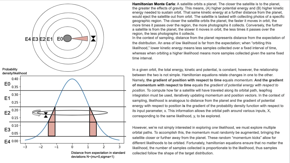
I made the below graphic to explain how I currently understand the HMC algorithm. I'd like verification from a subject matter expert if this understanding is or isn't correct. The text in the below slide is copied below for ease of access:

---

Hamiltonian Monte Carlo: A satellite orbits a planet. The closer the satellite is to the planet, the greater the effects of gravity. This means, (A) higher potential energy and (B) higher kinetic energy needed to sustain orbit. That same kinetic energy at a further distance from the planet, would eject the satellite out from orbit. The satellite is tasked with collecting photos of a specific geographic region. The closer the satellite orbits the planet, the faster it moves in orbit, the more times it passes over the region, the more photographs it collects. Conversely, the further a satellite is from the planet, the slower it moves in orbit, the less times it passes over the region, the less photographs it collects. In the context of sampling, distance from the planet represents distance from the expectation of the distribution. An area of low likelihood is far from the expectation; when “orbiting this likelihood,” lower kinetic energy means less samples collected over a fixed interval of time, whereas when orbiting a higher likelihood means more samples collected given the same fixed time interval. In a given orbit, the total energy, kinetic and potential, is constant; however, the relationship between the two is not simple. Hamiltonian equations relate changes in one to the other. Namely, the gradient of position with respect to time equals momentum. And the gradient of momentum with respect to time equals the gradient of potential energy with respect to position. To compute how far a satellite will have traveled along its orbital path, leapfrog integration must be used, iteratively updating momentum and position vectors. In the context of sampling, likelihood is analogous to distance from the planet and the gradient of potential energy with respect to position is the gradient of the probability density function with respect to its input parameter, x. This information allows the orbital path around various inputs, X, corresponding to the same likelihood, y, to be explored.
However, we’re not simply interested in exploring one likelihood, we must explore multiple orbital paths. To accomplish this, the momentum must randomly be augmented, bringing the satellite closer or further away from the planet. These random “momentum kicks” allow for different likelihoods to be orbited. Fortunately, hamiltonian equations ensure that no matter the likelihood, the number of samples collected is proportionate to the likelihood, thus samples collected follow the shape of the target distribution.

---

My question is - Is this an accurate way to think about how Hamiltonian Monte Carlo works?

Edit:

I've implemented in some code based on my understanding of the algorithm. It works for a gaussian with mu=0, sigma=1. But if I change sigma it breaks. Any insights would be appreciated.

import numpy as np
import random
import scipy.stats as st
import matplotlib.pyplot as plt
from autograd import grad

def normal(x,mu,sigma):
    numerator = np.exp((-(x-mu)**2)/(2*sigma**2))
    denominator = sigma * np.sqrt(2*np.pi)
    return numerator/denominator

def neg_log_prob(x,mu,sigma):
    num = np.exp(-1*((x-mu)**2)/2*sigma**2)
    den = sigma*np.sqrt(np.pi*2)
    return -1*np.log(num/den)

def HMC(mu=0.0,sigma=1.0,path_len=1,step_size=0.25,initial_position=0.0,epochs=1_000):
    # setup
    steps = int(path_len/step_size) -1 # path_len and step_size are tricky parameters to tune...
    samples = [initial_position]
    momentum_dist = st.norm(0, 1) 
    # generate samples
    for e in range(epochs):
        q0 = np.copy(samples[-1])
        q1 = np.copy(q0)
        p0 = momentum_dist.rvs()        
        p1 = np.copy(p0) 
        dVdQ = -1*(q0-mu)/(sigma**2) # gradient of PDF wrt position (q0) aka momentum wrt position

        # leapfrog integration begin
        for s in range(steps):
            p1 += step_size*dVdQ/2 # as potential energy increases, kinetic energy decreases
            q1 += step_size*p1 # position increases as function of momentum 
            p1 += step_size*dVdQ/2 # second half "leapfrog" update to momentum    
        # leapfrog integration end        
        p1 = -1*p1 #flip momentum for reversibility    
        
        #metropolis acceptance
        q0_nlp = neg_log_prob(x=q0,mu=mu,sigma=sigma)
        q1_nlp = neg_log_prob(x=q1,mu=mu,sigma=sigma)        

        p0_nlp = neg_log_prob(x=p0,mu=0,sigma=1)
        p1_nlp = neg_log_prob(x=p1,mu=0,sigma=1)
        
        # Account for negatives AND log(probabiltiies)...
        target = q0_nlp - q1_nlp # P(q1)/P(q0)
        adjustment = p1_nlp - p0_nlp # P(p1)/P(p0)
        acceptance = target + adjustment 
        
        event = np.log(random.uniform(0,1))
        if event <= acceptance:
            samples.append(q1)
        else:
            samples.append(q0)
    
    return samples

Now it works here:

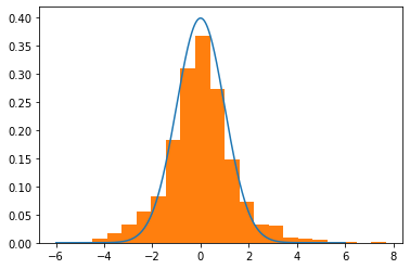
mu, sigma = 0,1
trial = HMC(mu=mu,sigma=sigma,path_len=2,step_size=0.25)

# What the dist should looks like
lines = np.linspace(-6,6,10_000)
normal_curve = [normal(x=l,mu=mu,sigma=sigma) for l in lines]

# Visualize
plt.plot(lines,normal_curve)
plt.hist(trial,density=True,bins=20)
plt.show()

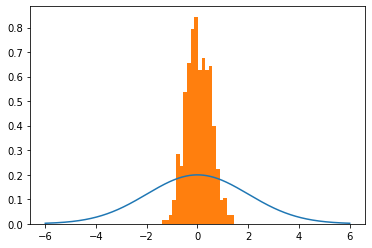
But it breaks when I change sigma to 2.

# Generate samples
mu, sigma = 0,2
trial = HMC(mu=mu,sigma=sigma,path_len=2,step_size=0.25)

# What the dist should looks like
lines = np.linspace(-6,6,10_000)
normal_curve = [normal(x=l,mu=mu,sigma=sigma) for l in lines]

# Visualize
plt.plot(lines,normal_curve)
plt.hist(trial,density=True,bins=20)
plt.show()

Any ideas? I feel like I'm close to "getting it".

Answer 1

Before answering the question about an intuitive way to think about Hamiltonian Monte Carlo, it's probably best to get a really firm grasp on regular MCMC. Let's set aside the satellite metaphor for now.

MCMC is useful when you want an unbiassed sample from a distribution where you only have something available which is proportional to the PDF, but not the PDF itself. This arises in (eg) physics simulations: the PDF is given by the Boltzmann distribution, p ~ exp(-E/kT), but the thing that you can calculate for any configuration of the system is E, not p. The constant of proportionality is not known, because the integral of exp(-E/kT) over the whole space of possible configuration is usually too difficult to calculate. MCMC solves that problem by doing a random walk in a specific way, where the probability of taking ("accepting") each step is related to the ratio of p values (the constant of proportionality cancels out). Over time, the distrubution of accepted samples from the random walk converges to the PDF that we want, without ever needing to explicitly calculate p.

Note that in the above, any method of taking random steps is equally valid, as long as the random walker can explore the whole space. The acceptance criterion guarantees that the selected samples converge to the real PDF. In practice, a gaussian distribution around the current sample is used (and the sigma can be varied so that the fraction of accepted steps stays relatively high). There would be nothing wrong in principle with taking steps from any other continuous distribution ("jumping distribution") around the current sample, although the convergence may be a lot slower.

Now, Hamiltonian Monte Carlo extends the physics metaphor by specifically trying to take steps in a direction which is more likely to be accepted than a gaussian step. The steps are what a leapfrog integrator would take, if it was trying to solve the motion of a system where the potential energy was E. These equations of motion also include a kinetic energy term, with a (not literally physical) "mass" and "momentum". The steps that the leapfrog integrator takes in "time" are then passed as proposals to the MCMC algorithm.

Why does this work? The gaussian MC takes steps the same distance in every direction with equal probability; the only thing that biases it towards more densely populated areas of the PDF is that steps in the wrong direction are more likely to be rejected. The Hamiltonian MC proposes steps both in the direction of E gradient, and the direction of accumulated motion in recent steps (direction and magnitude of the "momentum"). This enables faster exploration of the space, and also higher probability of reaching more densely populated regions faster.

Now, the satellite metaphor: I think this is not a very useful way to think about it. Satellites move in an exact orbit; what you have here is quite random, more like a particle of gas in a container with other particles. Each random collision gives you a "step"; over time the particle will be everywhere in the container with an equal probability (since the PDF here is equal everywhere, except the walls which represent very high energy / effectively zero PDF). Gaussian MCMC is like a effectively zero-mass particle doing a random walk (or non-zero mass particle in a relatively viscous medium): it will get there through brownian motion, but not necessarily fast. Hamiltonian MC is a particle with a non-zero mass: it may gather enough momentum to keep going in the same direction despite collisions, and so it may sometimes shoot from one end of the container to another (depending on its mass vs the frequency/magnitude of collisions). It would still bounce off the walls, of course, but it would in general tend to explore faster.