I have a multivariate data set of 12 sites, and 4 plots per site, except one site which only has three plots.
There two variables of interest: site_type, which is a property of a site, and ChaussB, which is a property of a plot.
genedat <- structure(list(
  site_type = structure(c(2L, 2L, 2L, 2L, 3L, 3L,  3L, 4L, 4L, 4L, 4L, 2L, 2L, 2L, 2L, 4L, 4L, 4L, 4L, 3L, 3L, 3L, 3L, 1L, 1L, 1L, 1L, 3L, 3L, 3L, 3L, 2L, 2L, 2L, 2L, 4L, 4L, 4L,  4L, 1L, 1L, 1L, 1L, 1L, 1L, 1L, 1L), .Label = c("CTRL", "OSP", "PMI", "SPS"), class = "factor"),
  site_num = structure(c(1L,1L, 1L, 1L, 2L, 2L, 2L, 3L, 3L, 3L, 3L, 4L, 4L, 4L, 4L, 5L, 5L, 5L, 5L, 6L, 6L, 6L, 6L, 7L, 7L, 7L, 7L, 8L, 8L, 8L, 8L, 9L, 9L,  9L, 9L, 10L, 10L, 10L, 10L, 11L, 11L, 11L, 11L, 12L, 12L, 12L, 12L), .Label = c("1", "2", "3", "4", "5", "6", "7", "8", "9", "10", "11", "12"),
  class = "factor"),
  ChaussB = c(7.425, 5.835,   5.777, 3.816, 8.284, 4.148, 0.712, 12.234, 6.558, 8.685, 5.304,  25.443, 6.022, 10.605, 17.453, 12.681, 4.381, 10.641, 8.478,  1.937, 5.504, 8.848, 1.445, 13, 7.379, 7.542, 13.942, 15.505,  13.876, 17.58, 7.322, 6.749, 5.007, 2.04, 5.063, 3.077, 9.61,  4.68, 8.991, 5.799, 2.798, 1.702, 0.683, 19, 8.39, 8.019, 9.706),
  Z1 = c(285.461, 207.466, 161.13, 162.624, 270.471, 107.079, 50.522, 164.952, 99.938, 181.951, 244.077, 157.943, 124.334,  201.943, 182.312, 171.339, 370.793, 145.31, 244.258, 218.455,  145.447, 270.552, 381.829, 315.364, 318.925, 159.2, 255.79, 141.412,  136.567, 109.169, 127.212, 305.645, 277.233, 140.165, 264.726, 119.308, 200.399, 106.124, 219.879, 252.846, 239.107, 266.249, 272.691, 245.463, 176.893, 251.416, 228.163),
  Z2 = c(76.481, 82.479, 59.776, 44.439, 43.108, 53.851, 87.029, 92.685, 98.246, 78.143, 70.159, 57.39, 82.761, 91.517, 80.155, 36.963, 79.341,  53.117, 77.068, 115.471, 78.491, 98.71, 69.541, 70.084, 48.926, 89.344, 64.351, 73.147, 44.431, 54.798, 77.864, 70.944, 83.23,  79.195, 81.495, 138.205, 112.615, 87.538, 81.669, 108.527, 78.925,  114.899, 61.416, 143.321, 117.269, 111.583, 55.279),
  pbsk3 = c(6.663, 17.307, 11.469, 12.851, 36.823, 46.956, 28.913, 55.045, 39.419,  58.338, 65.385, 97.297, 73.005, 11.543, 53.013, 40.485, 8.473, 49.538, 38.215, 27.183, 14.693, 28.688, 17.71, 9.976, 14.466,  4.395, 8.764, 116.219, 82.718, 85.201, 97.431, 8.263, 9.168,   6.056, 4.617, 60.954, 81.366, 72.638, 70.809, 4.872, 3.448, 0.896,  2.547, 4.572, 13.88, 10.459, 14.79),
  ef = c(74.583, 56.687, 52.155, 43.926, 52.836, 80.689, 79.235, 64.175, 63.455, 82.463, 83.243,  73.91, 66.312, 45.503, 71.731, 62.278, 64.739, 67.313, 89.245,  54.963, 43.247, 89.854, 50.678, 51.555, 73.532, 56.55, 58.86, 67.018, 71.244, 88.623, 74.962, 46.056, 69.064, 60.321, 72.253,  67.595, 73.161, 78.051, 63.705, 68.714, 82.995, 67.746, 44.37,  74.057, 60.539, 31.707, 51.561),
  Neith = c(7.535, 3.927, 3.647,  1.696, 8.863, 16.422, 11.33, 16.493, 18.186, 8.475, 16.635, 22.312, 5.624, 17.778, 20.342, 0.271, 1.711, 1.075, 0, 9.429, 0.306, 0.286, 1.332, 14.866, 0.093, 0.929, 4.241, 10.617, 12.96, 7.924, 7.466, 1.762, 1.709, 1.307, 1.02, 2.623, 14.468, 14.437, 13.101, 3.515, 1.818, 3.455, 9.414, 4.92, 7.361, 9.355, 1.543),
  msoA = c(0.208,  0.149, 0, 0, 0, 3.201, 17.085, 0, 12.879, 0.301, 0, 7.179, 15.91,  0.596, 1.393, 1.383, 0, 10.909, 0.979, 21.244, 0, 0, 0, 0, 0.092,  0.251, 0.139, 0.54, 2.932, 12.859, 0, 0, 0, 0, 1.368, 1.024, 5.467, 7.206, 0.319, 0.272, 0, 0, 0, 0, 0, 0, 0),
  Drm = c(26.657,  16.632, 26.695, 12.823, 15.28, 16.241, 15.313, 21.858, 10.588,  22.686, 25.015, 70.114, 14.031, 37.692, 31.842, 14.353, 21.307,   16.575, 19.949, 21.706, 11.353, 9.786, 12.777, 19.257, 25.263,   11.198, 29.731, 38.233, 31.191, 31.724, 20.978, 12.031, 27.106, 13.521, 19.873, 22.596, 20.086, 23.748, 22.056, 10.99, 25.798, 24.667, 26.718, 18.299, 25.383, 15.376, 15.916),
  Whal = c(7.571,  12.275, 5.446, 3.262, 29.145, 53.783, 22.482, 71.746, 44.422,   58.025, 47.542, 119.587, 24.33, 16.454, 77.451, 6.668, 11.578, 4.374, 11.752, 39.356, 19.197, 12.151, 3.35, 15.546, 7.742, 5.725,  18.717, 36.162, 41.111, 25.293, 22.038, 2.088, 6.439, 7.574,  5.54, 39.086, 45.556, 49.419, 33.35, 3.715, 10.993, 3.706, 6.926,  12.557, 18.441, 4.13, 7.415),
  Nock = c(7.751, 7.863, 17.935,  7.088, 7.134, 11.764, 8.457, 20.806, 15.75, 16.481, 10.3, 31.506,  8.831, 8.393, 12.915, 6.11, 5.004, 11.309, 11.001, 7.87, 1.562,  3.002, 0, 10.946, 10.122, 3.002, 3.433, 24.9, 14.014, 18.458,  17.227, 7.945, 7.428, 4.377, 7.417, 9.363, 16.04, 10.143, 5.904,  7.983, 4.357, 6.156, 11.373, 5.216, 12.634, 7.536, 6.739),
  dNor = c(0,  1.479, 0.268, 0, 1.807, 6.288, 0.729, 6.799, 1.448, 4.553, 5.276,   13.856, 1.799, 0, 1.271, 0, 0.344, 0, 0, 1.957, 0, 0.991, 0, 0, 0, 0, 0, 1.281, 1.937, 1.699, 2.541, 0, 0, 0, 0, 0.307, 7.611, 1.847, 2.125, 0, 0, 2.013, 0, 0, 0, 0, 0.513),
  rNor = c(12.375,  10.044, 6.229, 4.069, 13.416, 26.31, 28.969, 39.706, 17.511, 14.154, 21.506, 44.089, 12.276, 22.153, 36.964, 1.737, 1.615, 2.287, 0, 27.207, 1.881, 1.516, 1.272, 13.883, 0.866, 1.801,  5.971, 11.734, 13.156, 9.034, 8.395, 3.812, 2.792, 4.706, 1.59,  20.828, 14.984, 14.384, 18.532, 5.065, 2.486, 9.731, 10.364,  5.855, 15.134, 8.966, 7.05)), row.names = c(NA, -47L), class = "data.frame")
We can ordinate these data to see how they disperse by site_type:
library(vegan)
set.seed(14)
genNMDS <- metaMDS(genedat[,4:14], try=20, trymax=1000, k=2, maxit=200)
If we were do to any sort of permutation test on this, there would be an issue of pseudoreplication, because the sample size (n=47 plots) is inappropriate here because site_type is a property of site (n=12).
> envfit(genNMDS ~ site_type, data=genedat)

***FACTORS:

Centroids:
                NMDS1   NMDS2
site_typeCTRL -0.1382 -0.0674
site_typeOSP  -0.0227 -0.0366
site_typePMI   0.0761  0.0574
site_typeSPS   0.0910  0.0514

Goodness of fit:
              r2 Pr(>r)
site_type 0.2294  0.009 **
---
Signif. codes:  0 ‘***’ 0.001 ‘**’ 0.01 ‘*’ 0.05 ‘.’ 0.1 ‘ ’ 1
Permutation: free
Number of permutations: 999


> adonis(genedat[,4:14] ~ site_type, data=genedat)

Call:
adonis(formula = genedat[, 4:14] ~ site_type, data = genedat)

Permutation: free
Number of permutations: 999

Terms added sequentially (first to last)

          Df SumsOfSqs  MeanSqs F.Model      R2 Pr(>F)
site_type  3   0.33944 0.113148  3.8859 0.21329  0.003 **
Residuals 43   1.25205 0.029117         0.78671
Total     46   1.59149                  1.00000
---
Signif. codes:  0 ‘***’ 0.001 ‘**’ 0.01 ‘*’ 0.05 ‘.’ 0.1 ‘ ’ 1
We should really be considering sites as strata, and permuting entire sites, using the how() function in the permute package.
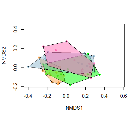
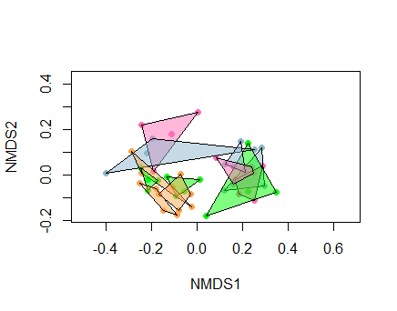
plot(genNMDS, type = "n")
points(genNMDS, display = "sites", col = colvec[genedat$site_type], pch=19)
ordihull(genNMDS, groups=genedat$site_num, col= colvec[c(2, 3, 4, 2, 4, 3, 1, 3, 2, 4, 1, 1)], draw="polygon")
library(permute)
h=with(genedat, how(within=Within(type="free"), plots=Plots(strata=site_num, type="free")))
But if we do so, as discussed in the permute::how() documentation and in this question we run into an error because we are missing a plot for one of the sites.
> envfit(genNMDS ~ site_type, data=genedat, perm=h)
Error in check(sn, control = control, quietly = quietly) :
  Design must be balanced if permuting 'strata'.
> adonis(genedat[,4:14] ~ site_type, data=genedat, perm=h)
Error in check(sn, control = control, quietly = quietly) :
  Design must be balanced if permuting 'strata'.
Question 1: Why must the design be balanced? I suspect it must have something to do with the number of possible ways you can permute a 4-plot site into a 3-plot site, and therefore each site_type group has a slightly different power associated with it. But I would appreciate a more extensive explanation.
Question 2: How can I assess the question of whether the site_types are significantly separating on either the ordination (envfit) or in the distance matrix (adonis) given the imbalance that precludes permuting by strata?
One solution I came up with is the average all plot data by site, and then evaluate on a data set of n=12 (without the subsampling).
library(dplyr)
genedatagg <- genedat %>% group_by(site_num, site_type) %>% summarize(across(is.numeric, mean))
set.seed(14)
aggNMDS <- metaMDS(genedatagg[,4:14], try=20, trymax=1000, k=2, maxit=200)
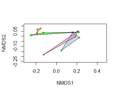
plot(aggNMDS, type = "n")
points(aggNMDS, display = "sites", col = colvec[genedatagg$site_type], pch=19)
ordihull(aggNMDS, groups=genedatagg$site_type,draw="polygon", col=colvec)
> envfit(aggNMDS ~ site_type, data=genedatagg)

***FACTORS:

Centroids:
                NMDS1   NMDS2
site_typeCTRL -0.1790  0.0570
site_typeOSP  -0.0530  0.0283
site_typePMI   0.1426 -0.0394
site_typeSPS   0.0894 -0.0459

Goodness of fit:
              r2 Pr(>r)
site_type 0.4593  0.143
Permutation: free
Number of permutations: 999

> adonis(genedatagg[,4:14] ~ site_type, data=genedatagg)

Call:
adonis(formula = genedatagg[, 4:14] ~ site_type, data = genedatagg)

Permutation: free
Number of permutations: 999

Terms added sequentially (first to last)

          Df SumsOfSqs  MeanSqs F.Model      R2 Pr(>F)
site_type  3   0.08214 0.027380  1.4614 0.35402  0.267
Residuals  8   0.14988 0.018735         0.64598
Total     11   0.23202                  1.00000
But this is not optimal if I simultaneously want to test ChaussB as this variable is a property of a plot, not a site (we would lose power for this variable by aggregating).
envfit(aggNMDS ~ site_type + ChaussB, data=genedatagg)
adonis(genedatagg[,4:14] ~ site_type + ChaussB, data=genedatagg)


