Working convention: Point $(0,1)$ is the upper left corner and corresponds to $0$ Recall (i.e. no Recall) and $1$ Precision (i.e. perfect Precision).
Regarding the first question:
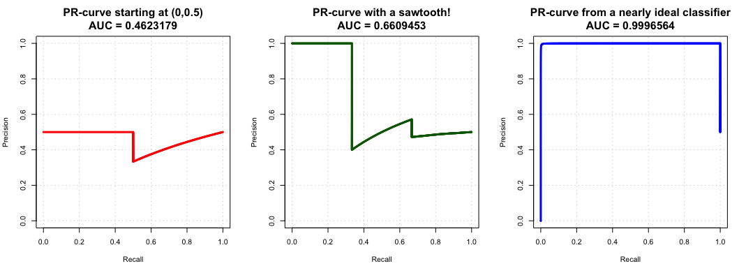
The start point can be at any point along $0$ or $\frac{1}{n_+}$ Recall, where the PR-curve start depends on the classifier performance. While we would hope that we will start at the point $(\frac{1}{n_+},1)$ and we will slow increase our Recall with little expense to Precision (i.e. we are very precise to begin with and slowly sacrifice Precision for Recall) that is not guaranteed at all. The obvious example is when we misclassify our "most probable" example of our test set. In that case we have both $0$-th Recall and $0$-th Precision, i.e. we start from point $(0,0)$. For example, in the left-most graph shown below (red line), we have an artificial example where we start at point $(0,0.5)$ because the first $\frac{N}{2}$ points are indistinguishable from each other. We "immediately" classify correctly some examples (i.e. we get TPs and thus non-zero Recall) but at the same time we get an equal number of FPs leading us at a $0.5$ Precision.
Please note, that in the case that no Positive examples are found (TPs or FPs), Precision is meaningless. There is not general rule on that what we do there. sklearn sets this to be $1$ that strictly for its convenience and explicitly says that these points "do not have a corresponding threshold". To that respect, in Davis & Goadrich (2006) the procedure of constructing a PR curve when presented with an algorithm returning probabilities is: "first find the probability that each test set example is positive, next sort this list and then traverse the sorted list in ascending order."; as such it is implied/suggested that for a probability that no example is positive, it makes no sense to construct a PR curve. In R PRROC::pr.curve does a similar thing where the origin is at $(0,0$) from the first positive example (example shown in pr3 below).
Side-note: in Python this leads in the slightly awkward situation of having Recall 0 with Precision 0 and 1 at the same time.
import numpy as np
from sklearn.metrics import precision_recall_curve
print(__doc__)

my_ytest = np.concatenate([np.array(['1'] * 50), np.array(['2'] * 50)])
my_yscore = np.concatenate([ [0.95], np.random.uniform(0.0, 0.5, 49),
                            np.random.uniform(0.5, 0.9, 50) ])
prec, recall, _ = precision_recall_curve(my_ytest, my_yscore, pos_label="2")
prec[recall==0]
# array([0., 1.])
Regarding the second question: Yes, the ideal classifier has AUCPR equal to 1. The only way to have an ideal classifier (i.e. performance that touches point $(1,1)$) but AUCPR less than $1$, is if we somehow moved towards $(1,1)$ while not already having perfect Precision (i.e. $y=1$). On occasion PR curves have the "sawtooth" shape (e.g. the middle graph shown below (dark green)), that suggests a significant jump in performance. That "tooth" though can never reach the point $(1,1)$ because by definition there are some misclassified points already. The "sawtooth effect" is due to us having a batch of correctly classified points, that helps us move both our Precision and Recall higher, followed by a batch of wrongly classified points that causes the sharp deep in Precision. To get the upward slope we increased our TP numbers while our FP & FN numbers remained the same but that does not mean though we removed our previously misclassified points; we can therefore never reach perfect Precision at $y=1$. For example in the right-most graph shown below (blue) a single point prohibits us from hitting $\text{AUCPR} = 1$; that misclassified FP point actually ranks higher than any other point in the positive class and thus forces our PR curve to start at $(0,0)$.
OK and some R code to see this first-handed:
library(PRROC)
N = 30000
set.seed(4321)

# The first N/2 points from each population are indistinguishable
pr0 <- pr.curve(scores.class0=c(rep(0.5, N/2), runif(n = N/2, max=0.4)),
                scores.class1=c(rep(0.5, N/2), runif(n = N/2, min=0.4, max = 0.49)),
                curve = TRUE)

# The [0.5, 0.7] space allows us to have the performance increase
pr1 <- pr.curve(scores.class0=c(runif(N/3, min=0.9, max=1.0),
                                runif(N/3, min=0.5, max=0.7),
                                runif(N/3, max=0.25)),
                scores.class1=c(runif(N/2, min=0.7, max=0.9),
                                runif(N/2, min=0.0, max=0.5)),
                curve=TRUE)

# The single point causes us to start from (0,0)
pr2 <- pr.curve(scores.class0=runif(n = N, min=0.999),
                scores.class1=c(1, runif(N-1, max=0.999)),
                curve = TRUE)


par(mfrow=c(1,3))
plot(pr0, legend=FALSE, col='red', panel.first= grid(),
     cex.main = 1.5, main ="PR-curve starting at (0,0.5)")
plot(pr1, legend=FALSE, col='darkgreen', panel.first= grid(),
     cex.main = 1.5, main ="PR-curve with a sawtooth!")
plot(pr2, legend=FALSE, col='blue', panel.first= grid(),
     cex.main = 1.5, main ="PR-curve from a nearly ideal classifier")


