What is a corresponding waiting time distribution if the number of events is negative binomial distributed

Question

For many distributions that describe the counts of events for a given time, we can have a corresponding distribution that describes the waiting time between events.

For instance, we can see the binomial distribution as the number of events that a coin flip is heads within some time $T$ where the distribution of the distance/time between such events is geometric distributed.

Is there a similar distribution of waiting time when the number of events is negative binomial distributed?

Answer 1

The negative binomial distribution has also the geometric distribution as waiting time.

The geometric distribution can be expressed in two ways:

with the domain $k \in \lbrace 1,2,3,\dots \rbrace$

$$f(k) = (1-p)^{k-1}p^k$$

and with the domain $k \in \lbrace 0,1,2,\dots \rbrace$

$$f(k) = (1-p)^kp^k$$

---

Intuition

Say you have the following coin flips

 result: H,  H,  T,  T,  H,  T,  H,  T,  T,  H,   H, ...

The binomial distribution:

• counts the number of heads

• untill a given number of flips have occured (untill a certain time has passes and each time flip te time advances by 1).

    result: H,  H,  T,  T,  H,  T,  H,  T,  T,  H,   H, ...
   n-flips: 1,  2,  3,  4,  5,  6,  7,  8,  9,  10, 11, ...
        dT: 1,  1,          3,      2,          3,   1, ...
  

You can see the geometric distribution as the distribution of the distance (number of flips) between successive heads (which is at minimum 1).

For instance the waiting times in the above string of heads and tails was 1, 1, 3, 2, 3, 1, ...

The negative binomial distribution:

• counts the number of heads

• untill a given number of tails have occurred.

    result: H,  H,  T,  T,  H,  T,  H,  T,  T,  H,   H, ...
   n-tails: 0,  0,  1,  2,  2,  3,  3,  4,  5,  5,   5, ...
        dT: 0,  0,          2,      1,          2,   0, ...
  

You can see the geometric distribution as the distribution of the distance (number of tails) between successive heads (which is one less than the case of the binomial distribution)

---

Example simulation

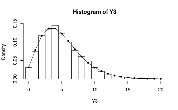
Image: simulated plotted as a histogram with modeled probability density as line and points

### function to sample based on waiting time
sample <- function(Te, p) {
  t = 0
  n = -1
  ### summing the time itteratively
  ### until the time 'Te' is surpassed
  while(t<Te){
    ti <- rgeom(1, p)
    t = t+ti
    n = n+1
  }
  n  ### return the number of itterations
}

### simulate
set.seed(1)
p = 0.5
Y <- replicate(10^4,sample(5, p))

### plot simulation histogram
hist(Y3, breaks = seq(-0.5,max(Y3)+0.5,1), freq = 0, xlim = c(0,20))
### plot model with line
lines(0:20,dnbinom(0:20,size = 5, prob = p)) 
points(0:20,dnbinom(0:20,size = 5, prob = p), cex = 0.7, pch = 21 , col = 1 , bg = 1)