Batch gradient descent versus stochastic gradient descent

Question

Suppose we have some training set $(x_{(i)}, y_{(i)})$ for $i = 1, \dots, m$. Also suppose we run some type of supervised learning algorithm on the training set. Hypotheses are represented as $h_{\theta}(x_{(i)}) = \theta_0+\theta_{1}x_{(i)1} + \cdots +\theta_{n}x_{(i)n}$. We need to find the parameters $\mathbf{\theta}$ that minimize the "distance" between $y_{(i)}$ and $h_{\theta}(x_{(i)})$. Let $$J(\theta) = \frac{1}{2} \sum_{i=1}^{m} (y_{(i)}-h_{\theta}(x_{(i)}))^{2}$$

Then we want to find $\theta$ that minimizes $J(\theta)$. In gradient descent we initialize each parameter and perform the following update: $$\theta_j := \theta_j-\alpha \frac{\partial J(\theta)}{\partial \theta_{j}} $$

What is the key difference between batch gradient descent and stochastic gradient descent?

Both use the above update rule. But is one better than the other?

Answer 1

The applicability of batch or stochastic gradient descent really depends on the error manifold expected.

Batch gradient descent computes the gradient using the whole dataset. This is great for convex, or relatively smooth error manifolds. In this case, we move somewhat directly towards an optimum solution, either local or global. Additionally, batch gradient descent, given an annealed learning rate, will eventually find the minimum located in it's basin of attraction.

Stochastic gradient descent (SGD) computes the gradient using a single sample. Most applications of SGD actually use a minibatch of several samples, for reasons that will be explained a bit later. SGD works well (Not well, I suppose, but better than batch gradient descent) for error manifolds that have lots of local maxima/minima. In this case, the somewhat noisier gradient calculated using the reduced number of samples tends to jerk the model out of local minima into a region that hopefully is more optimal. Single samples are really noisy, while minibatches tend to average a little of the noise out. Thus, the amount of jerk is reduced when using minibatches. A good balance is struck when the minibatch size is small enough to avoid some of the poor local minima, but large enough that it doesn't avoid the global minima or better-performing local minima. (Incidently, this assumes that the best minima have a larger and deeper basin of attraction, and are therefore easier to fall into.)

One benefit of SGD is that it's computationally a whole lot faster. Large datasets often can't be held in RAM, which makes vectorization much less efficient. Rather, each sample or batch of samples must be loaded, worked with, the results stored, and so on. Minibatch SGD, on the other hand, is usually intentionally made small enough to be computationally tractable.

Usually, this computational advantage is leveraged by performing many more iterations of SGD, making many more steps than conventional batch gradient descent. This usually results in a model that is very close to that which would be found via batch gradient descent, or better.

The way I like to think of how SGD works is to imagine that I have one point that represents my input distribution. My model is attempting to learn that input distribution. Surrounding the input distribution is a shaded area that represents the input distributions of all of the possible minibatches I could sample. It's usually a fair assumption that the minibatch input distributions are close in proximity to the true input distribution. Batch gradient descent, at all steps, takes the steepest route to reach the true input distribution. SGD, on the other hand, chooses a random point within the shaded area, and takes the steepest route towards this point. At each iteration, though, it chooses a new point. The average of all of these steps will approximate the true input distribution, usually quite well.

Answer 2

As other answer suggests, the main reason to use SGD is to reduce the computation cost of gradient while still largely maintaining the gradient direction when averaged over many mini-batches or samples - that surely helps bring you to the local minima.

1. Why minibatch works.

The mathematics behind this is that, the "true" gradient of the cost function (the gradient for the generalization error or for infinitely large samples set) is the expectation of the gradient $g$ over the true data generating distribution $p_{data}$; the actual gradient $\hat{g}$ computed over a batch of samples is always an approximation to the true gradient with the empirical data distribution $\hat{p}_{data}$. $$ \hat{g} = E_{\hat{p}_{data}}({\partial J(\theta)\over \partial \theta}) $$ Batch gradient descent can bring you the possible "optimal" gradient given all your data samples, it is not the "true" gradient though. A smaller batch (i.e. a minibatch) is probably not as optimal as the full batch, but they are both approximations - so is the single-sample minibatch (SGD).

Assuming there is no dependence between the $m$ samples in one minibatch, the computed $\hat{g}(m)$ is an unbiased estimate of the true gradient. The (squared) standard errors of the estimates with different minibatch sizes is inversely proportional to the sizes of the minibatch. That is, $$ {SE({\hat{g}(n)}) \over SE({\hat{g}(m)})} = { \sqrt {m \over n}} $$ I.e., the reduction of standard error is the square root of the increase of sample size. This means, if the minibatch size is small, the learning rate has to be small too, in order to achieve stability over the big variance. When the samples are not independent, the property of unbiased estimate is no longer maintained. That requires you to shuffle the samples before the training, if the samples are sequenced not randomly enough.

2. Why minibatch may work better.

Firstly, minibatch makes some learning problems from technically intractable to be tractable due to the reduced computation demand with smaller batch size.

Secondly, reduced batch size does not necessarily mean reduced gradient accuracy. The training samples many have lots of noises or outliers or biases. A randomly sampled minibatch may reflect the true data generating distribution better (or no worse) than the original full batch. If some iterations of the minibatch gradient updates give you a better estimation, overall the averaged result of one epoch can be better than the gradient computed from a full batch.

Thirdly, minibatch does not only help deal with unpleasant data samples, but also help deal with unpleasant cost function that has many local minima. As Jason_L_Bens mentions, sometimes the error manifolds may be easier to trap a regular gradient into a local minima, while more difficult to trap the temporarily random gradient computed with minibatch.

Finally, with gradient descent, you are not reaching the global minima in one step, but iterating on the error manifold. Gradient largely gives you only the direction to iterate. With minibatch, you can iterate much faster. In many cases, the more iterations, the better point you can reach. You do not really care at all weather the point is optimal globally or even locally. You just want to reach a reasonable model that brings you acceptable generalization error. Minibatch makes that easier.

You may find the book "Deep learning" by Ian Goodfellow, et al, has pretty good discussions on this topic if you read through it carefully.

Answer 3

To me, batch gradient resembles lean gradient. In lean gradient, the batch size is chosen so every parameter that shall be updated, is also varied independently, but not necessarily orthogonally, in the batch. For example, if the batch contains 10 experiments, 10 rows, then it is possible to form $2^{10-1} = 512$ independent columns. 10 rows enables independent, but not orthogonal, update of 512 parameters.

Answer 4

If you want to see the differences in a formula, this might help.

In above equation, m indicates the number of training data points.

In Batch Gradient Descent, As the yellow circle shows, in order to calculate the gradient of the cost function, we add up the cost of each sample. If we have 3 million samples, we have to loop through all 3 million samples or use the dot product.

def gradientDescent(X, y, theta, alpha, num_iters):
    """
    Performs gradient descent to learn theta
    """
    m = y.size  # number of training examples
    for i in range(num_iters):
        y_hat = np.dot(X, theta)
        theta = theta - alpha * (1.0/m) * np.dot(X.T, y_hat-y)
    return theta

Do you see np.dot(X.T, y_hat-y) above? That’s the vectorized version of “looping through (summing) all 3 million samples”.

Wait... just to move a single step towards the minimum, do we really have to calculate each cost 3 million times?

Yes. If you insist on using the batch gradient descent.

But if you use Stochastic Gradient Descent, you don’t have to!

In SGD, we use the cost gradient of ONE (1) example at each iteration, instead of adding up and using the costs of ALL examples.

Image Source

Answer 5

Imagine you are going down the hill to a valley of minimum height. You may use batch gradient descent to calculate the direction to the valley once and just go there. But on that direction you may have an up hill. It's better to avoid it, and this is what stochastic gradient descent idea is about. Sometimes is better to take small steps.

---

_{Just for the terminology direction batch gradient descent is not what you may intuitively think. This refers to the complete dataset pass per one iteration and in that context the entire dataset is called batch where we compute the average of the true gradient. Stochastic gradient descent is actually what we know as a multiple batches per iteration gradient descent update. This is why you may heard the word minibatch for the second.}

Answer 6

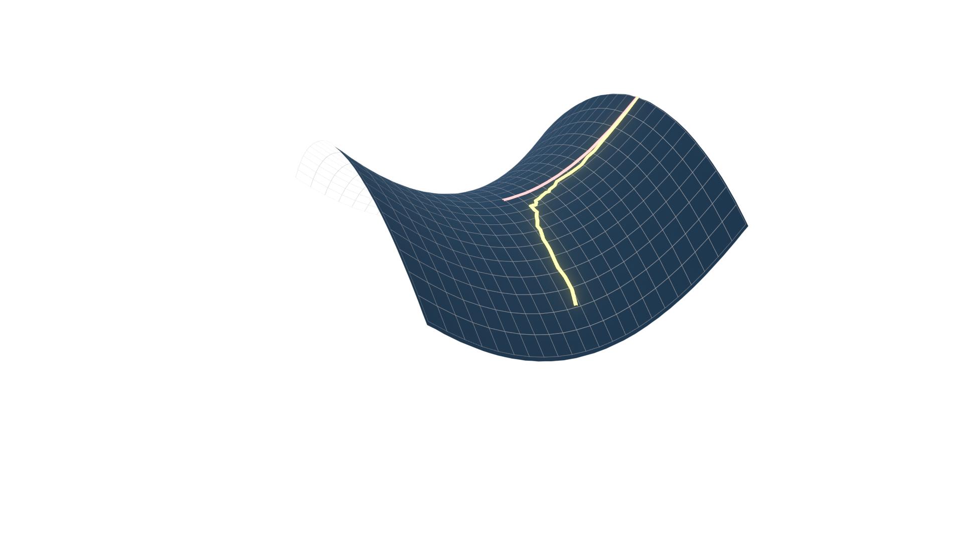
As mentioned in the above answers, the noise in stochastic gradient descent helps you escape "bad" stationary points. For example, you can see how gradient descent (in pink) gets stuck in a saddle point while stochastic gradient descent (in yellow) escapes it. This picture is taken from here.

Answer 7

Batch Gradient Descent(BGD):

• can do gradient descent with a whole dataset, taking only one step in one epoch. For example, a whole dataset has 100 samples(1x100), then gradient descent happens only once in one epoch which means model's parameters are updated only once in one epoch.
• 's pros:
  • The computation is stable(not fluctuated).
  • It's strong in noise(noisy data).
  • It gets an accurate value.
• 's cons:
  • It's not good at a large dataset because it takes much memory slowing down the computation.
  • It needs the repreparation of a whole dataset if you want to update a model.
  • It cannot easily escape local minima or saddle points.

Mini-Batch Gradient Descent(MBGD):

• can do gradient descent with splitted dataset(the small batches of a whole dataset) one small batch by one small batch, taking the same number of steps as the small batches of a whole dataset in one epoch. For example, the whole dataset which has 100 samples(1x100) is splitted into 5 small batches(5x20), then gradient descent happens 5 times in one epoch which means model's parameters are updated 5 times in one epoch.
• 's pros:
  • It's good at a large dataset because it takes small memory not slowing down the computation.
  • It's good at online learning. *Online learning is the way which a model incrementally learns from a stream of dataset in real-time.
  • It doesn't need the repreparation of a whole dataset if you want to update a model.
  • It can more easily escape local minima or saddle points than BGD.
• 's cons:
  • The computation is less stable than BGD.
  • It's less strong in noise(noisy data) than BGD.
  • It gets a less accurate value than BGD.

Stochastic Gradient Descent(SGD):

• can do gradient descent with every single sample of a whole dataset one sample by one sample, taking the same number of steps as the samples of a whole dataset in one epoch. For example, a whole dataset has 100 samples(1x100), then gradient descent happens 100 times in one epoch which means model's parameters are updated 100 times in one epoch.
• 's pros:
  • It's good at a large dataset because it takes small memory not slowing down the computation.
  • It's good at online learning.
  • It doesn't need the repreparation of a whole dataset if you want to update a model.
  • It can more easily escape local minima or saddle points than MBGD.
• 's cons:
  • The computation is less stable than MBGD.
  • It's less strong in noise(noisy data) than MBGD.
  • It gets a less accurate value than MBGD.