Are there better approaches than the weighted mean?

Question

If I have a data set where the distribution from which the data are drawn changes, for example in the following plot, the data set is comprised of four normal distributions with the same mean ($\mu = 0$) but different standard deviations:

If I wanted to get an average value for the data set, my instinct would be to calculate a weighted mean: $$\bar{\mu} = \frac{\sum_{i} w_{i} \mu_{i}}{\sum_{i} w_{i}}$$ where $\mu_{i}$ are the means of the individual distributions shown in the plot, and $w_{i} = 1 / (\sigma_{i} /\sqrt{n})^{2}$ are the weights, which can be used to compute a weighted standard-error: $${\rm{SE}} = \frac{1}{\sqrt{\sum_{i} w_{i}}}$$

I was wondering if there are better approaches where I could avoid binning or dividing the data up. One approach I have considered is considering the data as a mixed-distribution (mixed-normal distributions, with different $\sigma$) and performing a maximum-likelihood evaluation with the hypothesis $$G(x) = \sum_{i}\hat{w}_{i}g(x|\mu_{i}, \sigma_{i})$$ where ${w}_{i}$ are normalised weights and $g(x|\mu_{i}, \sigma_{i})$ are the component normal distributions.

I would then construct my weighted mean and standard error from the parameters of this MLE.

What I want to avoid is binning the data if possible, and assumptions based on where one distribution begins and ends.

---

The property I am measuring is from a normal distribution. I can say this with some certainty due to the physics of the problem. However due to laboratory conditions the standard deviation can fluctuate (the mean can also fluctuate but to a lesser extent -- the mean is always very close to 0). The scatter of the measurement can be stable for a few hours before changing. I have many datasets recorded over the course of month, so it seems reasonable to group the data by like-scatter and perform a weighted mean. However this requires me to make an assumption on group size, or what constitutes "like-scatter".

When I group data into like plots, Shapiro-Wilk tests and Q-Q plots all indicate that the data is indeed normally distributed, while autocorrelation tests imply randomness (no autocorrelation).

Answer 1

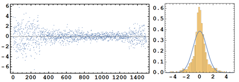
There seems to be a smooth dependence of variance on observation index, so you could try a joint modeling approach, see for instance Articles that work with covariates for mean, variance, and correlation simultaneously. Maybe also look into if there is autocorrelation (show us a plot!), and tell us what your data represents, and how it was obtained.

---

There are earlier post about estimation with estimated weights, for instance Determine weights in weighted least squares regression, and this list. A paper on this topic is available in JSTOR.

Carroll, Raymond J., et al. “The Effect of Estimating Weights in Weighted Least Squares.” Journal of the American Statistical Association, vol. 83, no. 404, 1988, pp. 1045–54. JSTOR, https://doi.org/10.2307/2290134. Accessed 6 Nov. 2022.

---

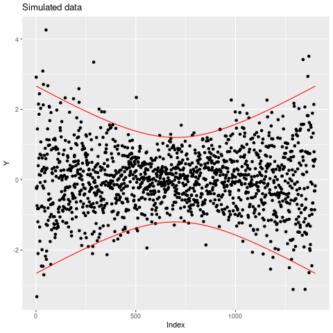
We can look at some simple simulations to see how much better we can do with a weighted mean, with data similar to yours. I will write simulation code (in R) that easily can be extended with other approaches. First I will show a dataset simulated similar to yours, with overlaid curves (red) of plus/minus two (known) standard deviations:

The optimal weights for the weighted mean is the inverse variance, which is known for the simulated data. In practive we must estimate the variance. That can be done in many ways, here I will use the R package gamlss, which implements joint estimation of mean and variance, in a framework which is an extension of the usual glm's (generalized linear models), in that we can also define link functions (and then a regression model) for the variance. I will define two models, one estimating a quadratic variance function (we simulated with a quadratic variance function), another with the variance modeled via a spline function. Both uses a log link function (and an identity link for the mean.) Then we simulate data as above 1000 times and estimates the mean by five methods:

1. unweighted mean
2. optimal weighted mean
3. weighted mean with weights estimated by gamlss with quadratic variance function
4. weighted mean with weights estimated by gamlss with spline variance function
5. weighted mean with weights from variance estimated by bins/buckets (I use 100 observations by bin)

and finally we present the squareroot of the mean square residual error around the known truth, zero:

m.unweighted  m.optweighted   m.bucket     m.gamlss0     m.gamlss1 
0.02416481    0.02160241      0.02175347   0.02149437    0.02152971    

It might be better to present this as relative efficiencies, that is, as a ratio of variances as compared to the optimal weights:

m.unweighted  m.optweighted   m.bucket     m.gamlss0     m.gamlss1 
1.2513028     1.0000000       1.0140346    0.9900230     0.9932804 

Note the small differences, but it seems that you can gain some by using, say, a spline variance model. The spline-based scheme is better that binning. For your data, I suspect there will be autocorrelation in time, which we have not modeled.

---

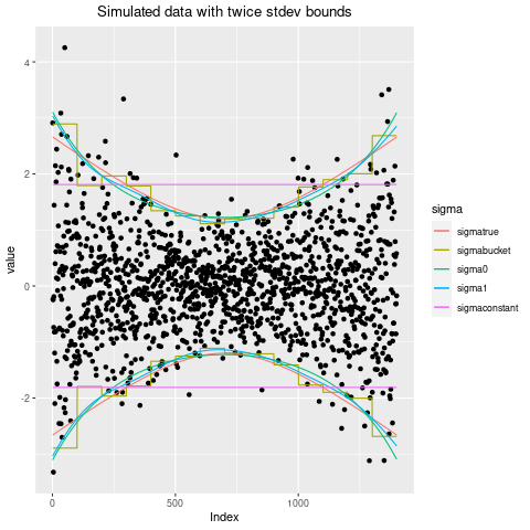
I will give some details and code, so the simulations can be adapted. First let us repeat the data plot, but with all the different standard deviations estimates given:

From this plot it is clear that the main step is to go from the constant variance model, with relatively small differences between the estimated variance function methods. I would go for the flexible spline model. So some code:

N <- 1400
Index <- 1:N

varfun <- function(trange) {
    ma <- 6; mi <- 0.6^2
    inds <- (trange - min(trange))/diff(range(trange))
    vars <- (0.25-inds*(1.0-inds))*(ma-mi) + mi
    vars
    }

set.seed(7*11*13)# My public seed
sigmatrue <- sqrt(varfun(Index))
Y <- rnorm(N, 0, sd=sigmatrue)

mydata <- data.frame(Y, Index, sigmatrue)

Using gamlss to estimate the model with a quadratic variance function:

library(gamlss)
mod0 <- gamlss::gamlss(Y  ~ 1, sigma.formula=  ~ Index + I(Index^2),
                       data= mydata)

sigma0 <- predict(mod0, what="sigma", type="response") 

The variable sigma0 contains the estimated standard deviations from this model, estimated jointly with the mean. The mean estimate can be read from the model summary:

 mod0

Family:  c("NO", "Normal") 
Fitting method: RS() 

Call:  gamlss::gamlss(formula = Y ~ 1, sigma.formula = ~Index +  
    I(Index^2), data = mydata) 

Mu Coefficients:
(Intercept)  
    0.01302  
Sigma Coefficients:
(Intercept)        Index   I(Index^2)  
  4.426e-01   -2.663e-03    1.899e-06  

 Degrees of Freedom for the fit: 4 Residual Deg. of Freedom   1396 
Global Deviance:     3467.21 
            AIC:     3475.21 
            SBC:     3496.19 

The estimated mean is the same as the weighted mean using inverse variance weights from the estimated variance function, as can be seen from

 weighted.mean(Y, (1/sigma0)^2)
[1] 0.01302066

The other spline model can be treated likewise so will not be given. Directly to the simulation code:

var_buckets <- function(Y, size) {
# If size do not divide length(Y) throw an error:
    n <- length(Y)
    stopifnot( n%%size == 0 )
    k <- n%/%size # Number of buckets
    vars <- numeric(n) ; len <- n/k
    for (i in 1:k) vars[((i-1)*len+1):(i*len)] <-
                       var(Y[((i-1)*len+1):(i*len)])
    return( vars )
    }

sigmabuckets <- sqrt(var_buckets(Y, 100))

B <- 1000
set.seed(7*11*13)# My public seed
sigmatrue <- sqrt(varfun(Index))
one_iter <- function() {
    mydat <- data.frame(Y=rnorm(N, 0, sd=sigmatrue), Index)
    mod0 <- gamlss::gamlss(Y  ~ 1, sigma.formula=  ~ Index + I(Index^2),
                       data= mydat)
    mod1 <- gamlss::gamlss(Y  ~ 1, sigma.formula=  ~ pb(Index),
                           data= mydat)   # pb uses CV for choosing df
    sigma0 <- predict(mod0, what="sigma", type="response")
    sigma1 <- predict(mod1, what="sigma", type="response")
    m.unweighted <- c(with(mydat, mean(Y)))
    m.optweighted <- c(with(mydat, weighted.mean(Y, (1/sigmatrue)^2)))
    m.gamlss0 <-  coef(mod0) ; names(m.gamlss0) <- NULL
    m.gamlss1 <-  coef(mod1) ; names(m.gamlss1) <- NULL
    sigmabucket <- with(mydat,  sqrt( var_buckets(Y, 100) ))
    m.bucket <- with(mydat, weighted.mean(Y, (1/sigmabucket)^2 ))
    return(c(m.unweighted=m.unweighted,
             m.optweighted=m.optweighted,
             m.bucket=m.bucket,  
             m.gamlss0=m.gamlss0,
             m.gamlss1=m.gamlss1))    
    }

simresults <- t(replicate(B, one_iter() ))