Median survival in Kaplan-Meier curve with plateau at .5

Question

Given a survival curve, to find the median one can visualize a line at 0.5 and then find the time at which the survival curve intersects with the line. But what if the Kaplan-Meier curve is horizontal at S(t)=0.5?

I´ve tried to come up with the solution by thinking of S(M)=0.5 and solving that equation for M. but it does not make sense to me. Is it possible to find an exact time point for the median survival, or will I get an interval?

Answer 1

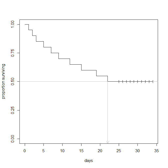
The median survival time is generally may be defined¹ as the shortest time at which the proportion surviving is $\le .5$ (for a more comprehensive overview, see: Finding median survival time from survival function). You need the Kaplan-Meier estimator to account for censoring correctly, but when you have that, you can read the median off the curve. Here is an example, coded in R:

library(survival)  # we'll need this package
times  = c( 1,  2,  3,  5,  7,  9, 12, 15, 19, 22, 
           25, 26, 27, 28, 29, 30, 31, 32, 33, 34 )
events = c( 1,  1,  1,  1,  1,  1,  1,  1,  1,  1,
            0,  0,  0,  0,  0,  0,  0,  0,  0,  0 )

windows()  # the KM plot
  plot(Surv(times, events), conf.int=FALSE, mark.time=TRUE, 
       yaxp=c(0,1,4), ylab="proportion surviving", xlab="days")
  segments(x0=-2, x1=22, y0=.5,   col="gray")
  segments(x0=34, x1=36, y0=.5,   col="gray")
  arrows(  x0=22, y0=.5, y1=-.04, col="gray", length=.1)

50% survive at least 22 days, so that's the median survival time. If you like, you can get R to compute it for you. Notice that the survival time is computed, as is the lower bound of a 95% confidence interval on the median survival time, but the upper bound cannot be computed in this case.

survfit(Surv(times, events)~1)
# Call: survfit(formula = Surv(times, events) ~ 1)
# 
#       n  events  median 0.95LCL 0.95UCL 
#      20      10      22      12      NA 

---

Although it's a much more advanced topic, you may wonder why the survival times are all censored after a certain point. It could be there there are two different processes at work, such that there is one distribution of survival times for some patients, and the other proportion may well die of something someday, but will never die of the cause under study. This phenomenon is the focus of cure rate models.

_{1. Another possibility is to define it as the time of the midpoint between the two middle events, if an even number.}