I have the following r code. I created a multiple linear regression model on a math_and_alcohol dataset. I can see in the summary of the model that the r-squared is .8279 which means the model explains 83% of the variability around the mean.
Here is a list of most of the predictors. They include things like gender, age, family size, mother's/father's educational status and job status, family and school support, travel distance, free time, how much time student spends going out, drinking during the week and drinking on the weekend, internet access, health, etc
  ..$ sex       : Factor w/ 2 levels "F","M": 1 1 1 1 1 2 2 1 2 2 ...
  ..$ age       : int [1:395] 18 17 15 15 16 16 16 17 15 15 ...
  ..$ famsize   : Factor w/ 2 levels "GT3","LE3": 1 1 2 1 1 2 2 1 2 1 ...
  ..$ Pstatus   : Factor w/ 2 levels "A","T": 1 2 2 2 2 2 2 1 1 2 ...
  ..$ Medu      : int [1:395] 4 1 1 4 3 4 2 4 3 3 ...
  ..$ Fedu      : int [1:395] 4 1 1 2 3 3 2 4 2 4 ...
  ..$ Mjob      : Factor w/ 5 levels "at_home","health",..: 1 1 1 2 3 4 3 3 4 3 ...
  ..$ Fjob      : Factor w/ 5 levels "at_home","health",..: 5 3 3 4 3 3 3 5 3 3 ...
  ..$ traveltime: int [1:395] 2 1 1 1 1 1 1 2 1 1 ...
  ..$ studytime : int [1:395] 2 2 2 3 2 2 2 2 2 2 ...
  ..$ failures  : int [1:395] 0 0 3 0 0 0 0 0 0 0 ...
  ..$ schoolsup : Factor w/ 2 levels "no","yes": 2 1 2 1 1 1 1 2 1 1 ...
  ..$ famsup    : Factor w/ 2 levels "no","yes": 1 2 1 2 2 2 1 2 2 2 ...
  ..$ activities: Factor w/ 2 levels "no","yes": 1 1 1 2 1 2 1 1 1 2 ...
  ..$ nursery   : Factor w/ 2 levels "no","yes": 2 1 2 2 2 2 2 2 2 2 ...
  ..$ higher    : Factor w/ 2 levels "no","yes": 2 2 2 2 2 2 2 2 2 2 ...
  ..$ internet  : Factor w/ 2 levels "no","yes": 1 2 2 2 1 2 2 1 2 2 ...
  ..$ romantic  : Factor w/ 2 levels "no","yes": 1 1 1 2 1 1 1 1 1 1 ...
  ..$ famrel    : int [1:395] 4 5 4 3 4 5 4 4 4 5 ...
  ..$ freetime  : int [1:395] 3 3 3 2 3 4 4 1 2 5 ...
  ..$ goout     : int [1:395] 4 3 2 2 2 2 4 4 2 1 ...
  ..$ Dalc      : int [1:395] 1 1 2 1 1 1 1 1 1 1 ...
  ..$ Walc      : int [1:395] 1 1 3 1 2 2 1 1 1 1 ...
  ..$ health    : int [1:395] 3 3 3 5 5 5 3 1 1 5 ...
  ..$ absences  : int [1:395] 6 4 10 2 4 10 0 6 0 0 ...

math_grade_model <- lm(G3 ~ ., math_and_alcohol)
summary(math_grade_model)
summary(math_grade_model)$r.squared
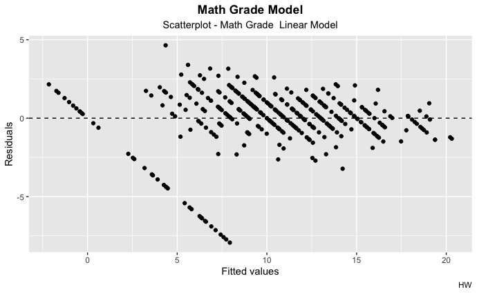
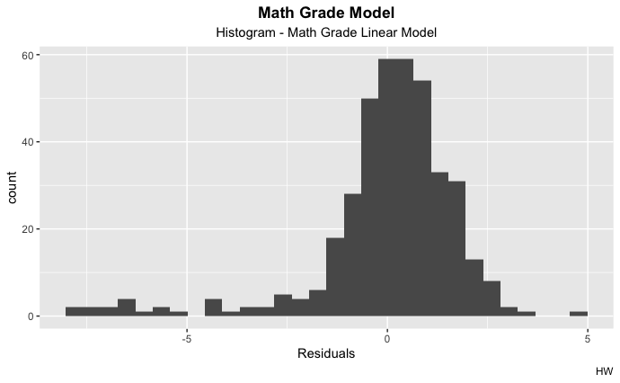
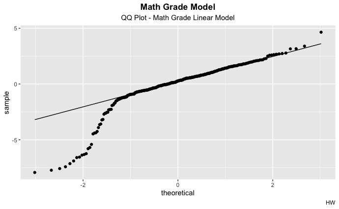
I now want to assess if this linear model is a good model. So I plotted the fitted values against the residuals. I also made a histogram of the residuals and I made a qq plot. I've been doing some reading and these are suggestions I have found.
My problem is I don't have any idea how to read these graphs!
The histogram looks a little left-skewed to me but mostly normal I think? The qq plot looks like a straight line except there's a serious tail on the left side. I have no idea how to understand the fitted values versus the residuals.
If anyone could help I would really appreciate it!
ggplot(data = math_grade_model, aes(x = .fitted, y = .resid)) +
    geom_point() +
    geom_hline(yintercept = 0, linetype = "dashed") +
    xlab("Fitted values") +
    ylab("Residuals") +
    labs(title = "Math Grade Model", subtitle = "Scatterplot - Math Grade  Linear Model") +
  theme(plot.title = element_text(hjust = 0.5, face = "bold")) +
  theme(plot.subtitle = element_text(hjust = 0.5)) +
  labs(caption = "HW")

ggplot(data = math_grade_model, aes(x = .resid)) +
  geom_histogram() +
  xlab("Residuals") +
  labs(title = "Math Grade Model", subtitle = "Histogram - Math Grade Linear Model") +
  theme(plot.title = element_text(hjust = 0.5, face = "bold")) +
  theme(plot.subtitle = element_text(hjust = 0.5)) +
  labs(caption = "HW")

ggplot(data = math_grade_model, aes(sample = .resid)) +
  stat_qq() + stat_qq_line() +
  labs(title = "Math Grade Model", subtitle = "QQ Plot - Math Grade Linear Model") +
  theme(plot.title = element_text(hjust = 0.5, face = "bold")) +
  theme(plot.subtitle = element_text(hjust = 0.5)) +
  labs(caption = "HW")
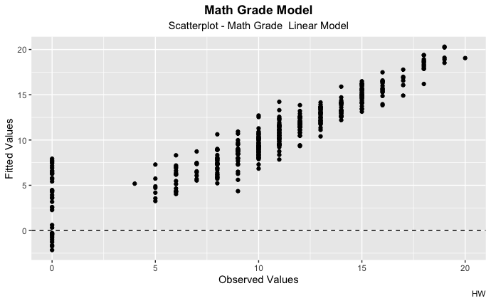
@Nick Cox I added another graph as you suggested. Now I've encountered a little bit of a coding question -- I think what I'm doing here is putting G3 on the x axis and then the fitted values from the model on the y-axis. I've never created this kind of graph before. Is this what you were picturing?
ggplot(data = math_grade_model, aes(x = math_and_alcohol$G3, y = .fitted)) +
    geom_point() +
    geom_hline(yintercept = 0, linetype = "dashed") +
    xlab("Observed Values") +
    ylab("Fitted Values") +
    labs(title = "Math Grade Model", subtitle = "Scatterplot - Math Grade  Linear Model") +
  theme(plot.title = element_text(hjust = 0.5, face = "bold")) +
  theme(plot.subtitle = element_text(hjust = 0.5)) +
  labs(caption = "HW")


