Elementary explanation of Gaussian Processes

Question

I'm learning of Gaussian Processes (GP) in the context of Bayesian Optimization (BO), where a surrogate function is learned to approximate the reward signal then a (hopefully) global optima is selected. Because GP are the backbone of BO, I'd like to get a better feel for what it's all about. Thus far, I've heard two explanations:

1. GPs are distributions over functions.
2. GPs are spline regression on steroids (instead of a supplied number of nodes, it's assumed an infinite number or at least one per observed point.)

These definitions don't seem to agree with one another; however, there's one thing they agree on: The kernel choice and hyperparameters are the most important elements of the GP.

Here's how I currently understand GPs:

• A GP receives some input data and initializes a "need" for several normal distributions (one over each observation.)
• the GP randomly samples distribution parameters for each observation
• The kernel, which largely regulates the cohesion of adjacent observation's distributions, evaluates the goodness of fit.
• This process repeats over and over until it converges on a posterior (of posteriors over each observation).

Could someone comment on how far this is off from reality? (If quite far, please provide an explanation.)

Answer 1

A stochastic process $X(t), t \in T$ is a Gaussian process (GP) if $\sum_i a_i X(t_i)$ is a Gaussian random variable for any such linear combination. Equivalently, it is a GP if all its finite-dimensional distributions are (multivariate) Gaussian, that is $(X(t_1),X(t_2),\dots,X(t_n))$ is Gaussian for any choice of $\{t_i\}$. Usually, one in addition requires that the sample path $t \mapsto X(t)$ be continuous. This way you can view a GP as a random function in $C(T)$ the space of all continuous functions on $T$.

A GP is characterized by a mean function $\mu: T \to \mathbb R$ and a covariance kernel $K$ (a positive semi definite function from $T \times T$ to $\mathbb R$) with the property that $\mathbb E [X(t)] = \mu(t)$ for all $t \in T$ and $$\text{cov}\big(\mathbf X) = (K(t_i,t_j))_{i,j=1}^n$$ where $\mathbf X = (X(t_1),X(t_2),\dots,X(t_n))$ and this holds for any choice of $\{t_1,\dots,t_n\} \subset T$ and any $n \ge 1$. Note that $\mu$ and $K$ effectively specify all those finite-dimensional normal distributions we talked about before.

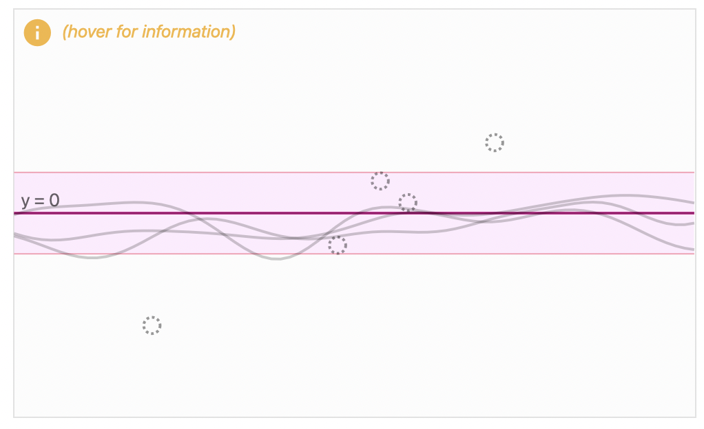
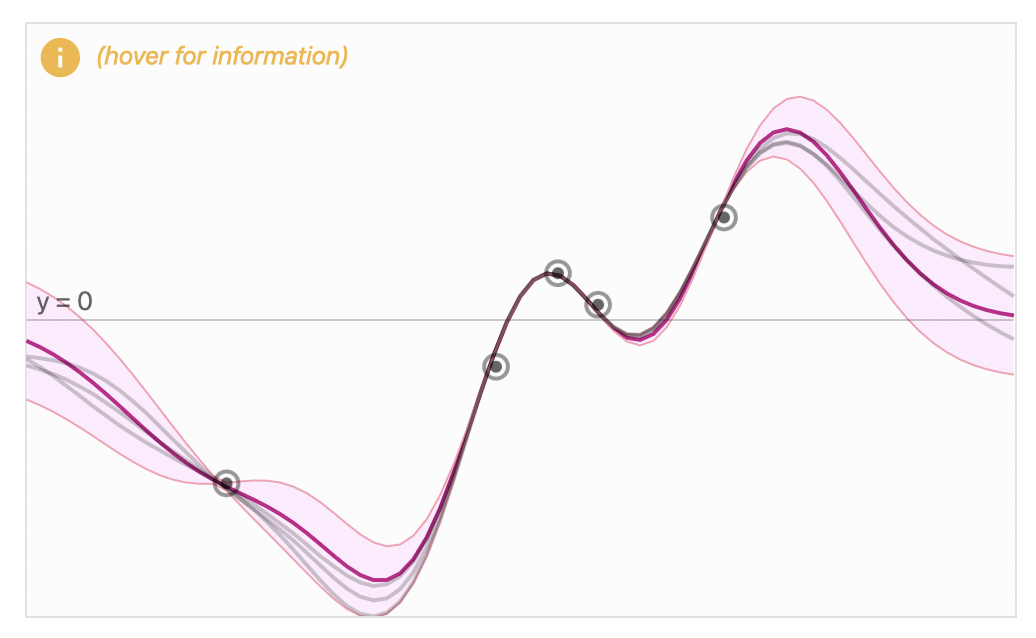
This is all good, but what does a GP look like? I mean, how do we even sample from a GP and what do the functions we sample from look like? How can we output an entire function every time we sample a single element from GP?

---

Representation

There is a very powerful result that allows us to give a nice answer to this question. To make it simple, I am not going to worry about mathematical rigor that much (maybe a little bit!). Here are a couple of observations:

• Associated to every kernel function $K(\cdot,\cdot)$, there is a unique reproducing kernel Hilbert space (RKHS), call it $H$. Let's not worry what RKHS means, it is just a deterministic space of "nice" functions. We can view $H$ as a subset of the $L^2$ space of functions on $T$.

• Thus associated to every GP, there is an RKHS determined by its covariance kernel. It turns out that the closure of $H$ (in $C(T)$) is the support of the GP, that is, $P( X \in \bar H) = 1$. We will never observe anything outside $\bar H$ when we sample from the GP.

• Let $\{\phi_j\}_{j \in \mathbb N}$ be a complete orthonormal system of eigenfunctions of the kernel matrix $K(\cdot,\cdot)$ (in $L^2$) and $\{\lambda_j\}_{j \in \mathbb N}$ the corresponding nonzero eigenvalues. We assume they are ordered as follows: $$ \lambda_1 \ge \lambda_2 \ge \lambda_3 \ge ... $$ and they are all nonnegative (a consequence of positive semi-definiteness.) If $H$ is infinite-dimensional, this sequence will also be infinite.

You might have heard of the Mercer's theorem which gives an expansion of the kernel in terms of these: $$ K(s,t) = \sum_{j=1}^\infty \lambda_j \phi_j(s) \phi_j(t). $$

• It turns out that the associated GP also has an expansion in terms of those eigenfunctions: Then, almost surely $$ X(t) = \mu(t) + \sum_{j=1}^\infty \sqrt{\lambda_j} g_j \phi_j(t). \quad (*) $$ where $g_i \sim N(0,1), i =1,2,3,\dots$ i.i.d. standard normal variables. This is called a Karhunen–Loève expansion. Since $\lambda_j \to 0$ as $j \to \infty$, you can truncate this series to some large value of $N$ and get a good approximation. Basically, a GP is a linear combination of these eigenfunctions with random weights $\sqrt{\lambda_j} g_j$ (which are drawn independently from a Gaussian distribution with zero mean and variance $\lambda_j$). You can think of these eigenfunctions as the directions of variation of the GP. There is more variability along $\phi_1$ followed by $\phi_2$ and so on. (Think of it like PCA in infinite dimensions.)

Representation (*) is good enough for understanding and you can just stop here. But the story doesn't end here. See the end of this post. To practically sample from the GP, find $\{\phi_j\}$ and $\lambda_j$, draw $\{g_j\}$ as i.i.d. standard normal variables and form $X(t) \approx \sum_{j=1}^N \sqrt{\lambda_j} g_j \phi_j(t)$ for some large enough $N$.

Example

Consider the Brownian motion on $[0,1]$ which is a centered sample-path-continuous GP with covariance matrix $\mathbb E [X(t) X(s)] = \min\{t,s\}$ for all $s,t \in [0,1]$. The eigenvalues and eigenfunctions are given by (see Example 12.23 in Wainwright's book) $$ \phi_j(t) = \sin \frac{(2j-1)\pi t}{2}, \quad \lambda_j = \Big( \frac{2}{(2j-1)\pi}\Big)^2. $$ Note that $\lambda_j \to 0$ as $j \to \infty$. Then, if you believe the K-L result, we can give a explicit construction of the Brownian motion as follows: $$ X(t) = \sum_{j=1}^\infty \frac{2 g_j}{(2j-1)\pi} \, \sin \left( \frac{(2j-1)\pi t}{2}\right) = \sum_{k \; \text{odd}} \frac{2 g_k}{k\pi} \, \sin \left( \frac{k\pi t}{2}\right). $$ where $g_1, g_2, g_3, \dots \stackrel{\text{i.i.d.}}{\sim} N(0,1)$.

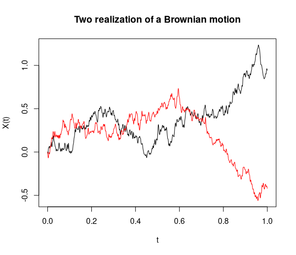
Here is some code to draw two samples from this random function:

tvec = seq(0,1, length.out = 1000)
N = 500
set.seed(125)

g1 = rnorm(N)
g2 = rnorm(N)

X_realization = function(tvec, g) {
   sapply(tvec, function(t) sum( sapply(1:N, function(j) 2*g[j]*sin((2*j-1)*pi*t/2)/(pi*(2*j-1)))) )
}

Xs1 = X_realization(tvec, g1)
Xs2 = X_realization(tvec, g2)

yrange = range(cbind(Xs1, Xs2))

plot(tvec, Xs1, type="l", ylim = yrange, main = "Two realizations of a Brownian motion", xlab = "t", ylab = "X(t)")
lines(tvec, Xs2, col="red")

And the resulting plot:

---

The rest of the story

It turns out that any complete orthonormal system of $H$ will do. So if you pick any sequence of functions $\{h_j\}$ that are orthonormal in $H$ and their closure spans the entire $H$, then, almost surely $$ X(t) = \sum_{j=1}^\infty g_j h_j, $$ where $\{g_j\}$ is some i.i.d. $N(0,1)$ sequence. This gives much flexibility in representing a GP and some basis might work better than the other in a specific application. (See Theorem 2.6.10 in Giné and Nickl's book).

---

In finite dimensions

EDIT: Since this post got some attention, let me add this too. The K-L expansion mentioned above is not unfamiliar to you if you have thought about how to sample a general multivariate Guassian vector $\mathbf x \sim N(\mu, \Sigma)$. What you would generally do is to write $\mathbf x = (x_i) = \mu + \Sigma^{1/2} \mathbf z \in \mathbb R^n$ where $\mathbf z \sim N(0,I)$ that is $\mathbf z = (z_i)$ with $z_1,\dots,z_n$ i.i.d. $\sim N(0,1)$ and $\Sigma^{1/2}$ is the matrix square root of $\Sigma$.

Another closely related approach is to perform eigen-decompisition on $\Sigma = U \Lambda U^T$ where $U = [\mathbf u_1 \mid \mathbf u_2 \mid \cdots \mid \mathbf u_n]$ is an orthogonal matrix whose columns are the eigenvectors of $\Sigma$ and $\Lambda = \text{diag}(\lambda_i)$ is the diagonal matrix of the corresponding eigenvalues. Then, we can generate $\mathbf x = \mu + U \Lambda^{1/2} \mathbf z$ (verify that this has the right distribution!). If you expand this equation you get $$ \mathbf x = \mu + \sum_{i=1}^n \sqrt{\lambda_i} z_i \mathbf u_i $$ which is just the finite-dimensional analog of the K-L expansion.

Answer 2

You are given points sampled from a function, that is not known, this is your data. Traditional curve fitting algorithms would try to find a function that fits the data the best. Gaussian process learns distribution over functions, i.e. you could sample from this distribution the functions that are consistent with the data. This distribution is defined in terms of mean function and covariance function, they are defined in terms of kernels. Kernel can be thought as a measure of similarity between points, so it forces the Gaussian process functions to be more similar for points that are similar to each other, and can be dissimilar for points that are less similar to each other.

When using Gaussian processes in optimization, we use it as a surrogate model, so instead of optimizing the target function, we optimize the function approximated by Gaussian process. We do this when it is expensive to evaluate the target function, for example, it is a neural network that is expensive and takes long to train. Instead we approximate the function. Since Gaussian process, because of being defined in terms of kernels, it is more uncertain for the areas where it saw less data and more certain in areas with more data. Thanks to this, you can optimize, or sample from the distribution, by taking into consideration the uncertainty. You want to explore areas that you are uncertain about.

Answer 3

I found this article very helpful towards building an intuition of GPs.

The mean and covariance functions you define for your prior distributions sets up the distribution that you can sample functions from, where the covariance affects the shape (wiggliness, trend, periodicity) of the functions.

Given observation points you use define a conditional distribution which now must pass through (or close to) your observation points. So if you have a observed points $Y$, and you are interested in the distribution of $X$ given $Y$ and you have assumed a Gaussian prior joint distribution with mean $\begin{pmatrix} \mu_X & \mu_Y \end{pmatrix}^\top$ and covariance matrix $\begin{pmatrix} \Sigma_{XX} & \Sigma_{XY} \\ \Sigma_{YX} & \Sigma_{YY}\end{pmatrix}$, the conditional distribution given the observations $Y$, $X|Y$ is given by

$$X|Y \sim \mathcal{N} (\mu_X + \Sigma_{XY}\Sigma_{YY}^{-1}(Y-\mu_Y), \Sigma_{XX} - \Sigma_{XY}\Sigma_{YY}^{-1}\Sigma_{YX}).$$

This distribution now looks more like this:

Once again it is a distribution, so functions can be sampled from it.

I also found this YouTube video helpful for building an intuition for kernel functions effect on shape.

(Images used from this article)