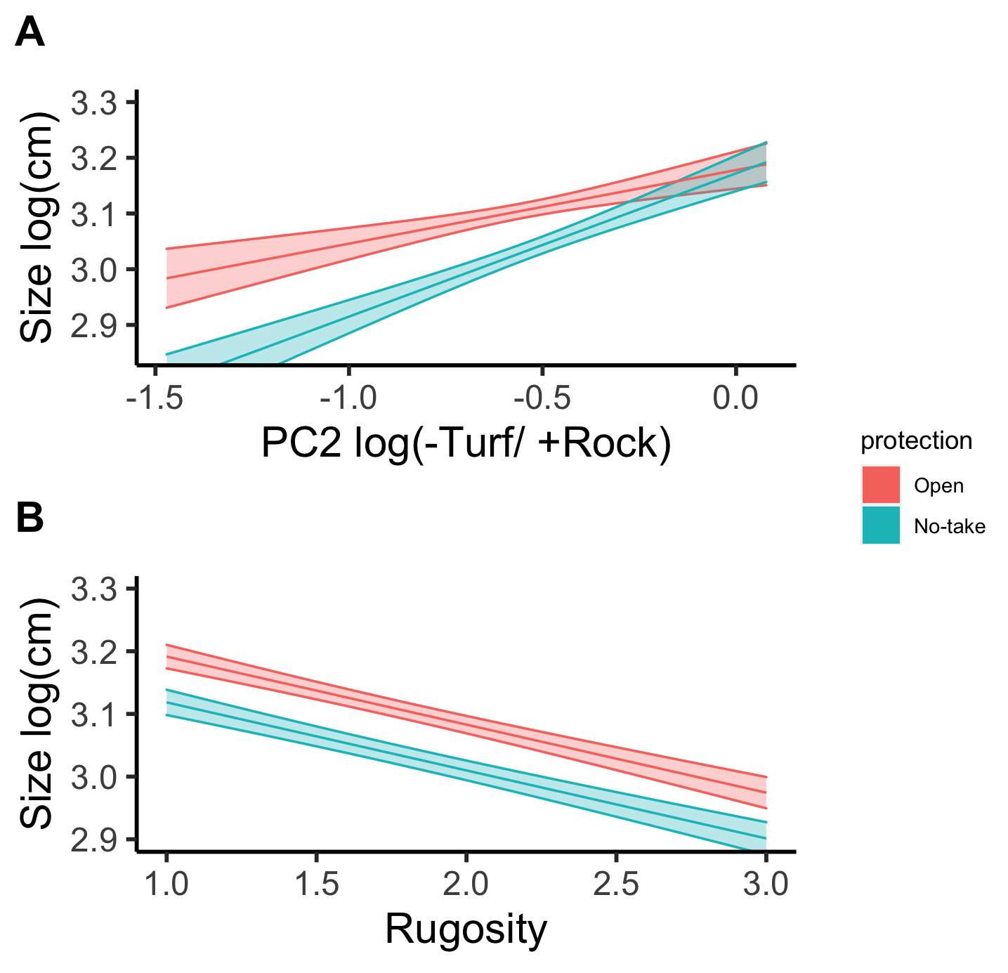
I am doing a multiple regression to predict average sizes of fish between areas protected from fishing and areas open to fishing. The model also takes into account habitat parameters which are the other variables (log.comp2 + rugosity). This model was the best according to AIC. log(size) transformation was used to normalize data.
mtar <- glm(log(size) ~ log.comp2 + rugosity + protection + log.comp2:protection, tar, family = "gaussian")
The output for summary(mtar) shows no significant difference for protection:
                             Estimate Std. Error t value Pr(>|t|)
(Intercept)                  3.370952   0.022943 146.928  < 2e-16 ***
log.comp2                    0.132060   0.028386   4.652 3.48e-06 ***
rugosity                    -0.108574   0.008749 -12.410  < 2e-16 ***
protectionNo-take           -0.005873   0.023595  -0.249  0.80346
log.comp2:protectionNo-take  0.125109   0.039544   3.164  0.00158 **
---
Signif. codes:  0 ‘***’ 0.001 ‘**’ 0.01 ‘*’ 0.05 ‘.’ 0.1 ‘ ’ 1

(Dispersion parameter for gaussian family taken to be 0.05726864)

    Null deviance: 139.63  on 2192  degrees of freedom
Residual deviance: 125.30  on 2188  degrees of freedom
AIC: -41.526
but the graph shows clear differences:

How can I interpret this?
