0
$\begingroup$

Let's say I have some value y for the first 7 days (day). I want to predict sum(y) after n days (a couple of weeks) and also get its distribution. (Note that days are already logged and scaled (scale(log(day))).

I'm interested in the Bayesian approach (I already found the same problem solved by frequentists) and I would appreciate an intuitive explanation and, if possible, solve it with as little math as possible (I prefer to simulate.:)). I don't mind if you use any other R package to implement the solution (tidybayes, ...) or just explain it.

library(rethinking)

# both columns are already logged and normalized - the reason days are not  integers
data <- tibble::tribble(
    ~day,                 ~y,
    -1.77840188804283,   1.59343897400421,
    -0.766238080609954,   1.26984673633088,
    -0.174160208674574, -0.369170057608193,
    0.245925726822919,  -0.65694469801144,
    0.571769693063722, -0.523623000175519,
    0.838003598758299, -0.924816393618227,
    1.06310115868241, -0.388731560921705
)

model <- quap(
    alist(
        y ~ dnorm(mu, sigma),
        mu <- a + b * day,
        a ~ dnorm(0, 0.1),
        b ~ dnorm(-1, 0.5),
        sigma ~ dnorm(0, 0.2)
    ),
    data = data
)

How to get the distribution of sum of predictions? This is: how is distributed sum(y) for the first n days?

$\endgroup$
4
  • $\begingroup$ You posted a Bayesian model description. What then is the question? $\endgroup$
    – Bernhard
    Commented Jan 17, 2021 at 20:23
  • $\begingroup$ How to get the distribution of sum of predictions? This is: how is distributed sum(y) for the first n days? $\endgroup$ Commented Jan 17, 2021 at 20:42
  • 1
    $\begingroup$ I'd get what "for the first n days" meant if days was discrete, e. g. ranged from 1:7, but with the given days in between -1.78 and 1.063 it appears to be some continuous value and those do not have first n values. $\endgroup$
    – Bernhard
    Commented Jan 18, 2021 at 10:28
  • $\begingroup$ I applied log(day) and normalized them afterward. Sorry if I wasn't clear. $\endgroup$ Commented Jan 18, 2021 at 10:38

2 Answers 2

1
$\begingroup$

As mentioned in the comment, the first n days in normalized days are disturbing to me, so I'd like to stay with discrete days. The data then becomes:

data <- data.frame(day = 1:7, y = c(-1.77840188804283, -0.766238080609954, -0.174160208674574, 
                                    0.245925726822919, 0.571769693063722, 0.838003598758299, 1.06310115868241))
plot(data$day, data$y)

Judging from your code you want to fit Bayesian linear regression to those data.

I choose a simple to perform way for that with sensible priors set automatically from the rstanarm package:

library(rstanarm)
model <- stan_glm(y ~ day, data = data, family = "gaussian")
plot(model)

posterior <- as.data.frame(model)

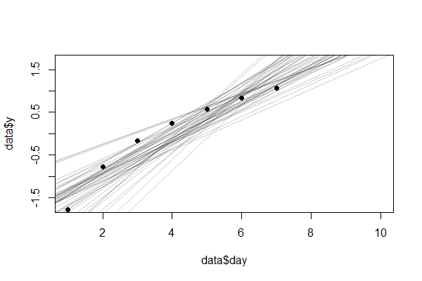
That will draw 4000 linear regression lines from the posterior distribution, the intercepts and slopes of which you find in posterior. This will plot the data and a sample of 50 of those regression lines:

plot(data$day, data$y, pch = 16)
for(i in 1:50){
  abline(posterior[i, 1], posterior[i, 2], col = alpha("black",.2))
}

enter image description here

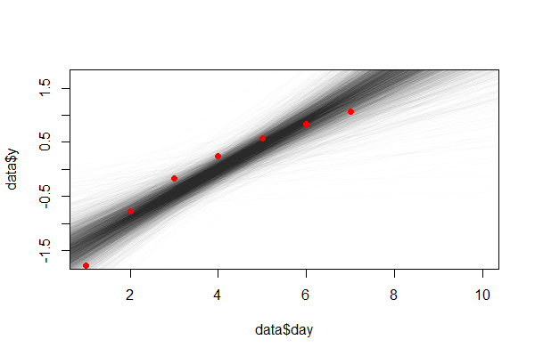
Or for all 4000 like this:

plot(data$day, data$y, xlim = c(1,10), ylim = c(-1.7, 1.7))
for(i in 1:4000){
  abline(posterior[i, 1], posterior[i, 2], col = alpha("black",.01))
}
points(data$day, data$y, pch = 16, col = "red")

enter image description here

Now, we can easily see how a linear regression is not the best way to predict data for the future and how all these regression lines will predict values that are to large, but model choice is not the topic of this question so we go on. (Probably this is because I did not use log-transformed days -- check that with the real data).

We can take each of these 4000 lines or a random sample of them in order to predict the sum(y) over the next n days, like for the days 8:12:

interval = 8:12
sums <- numeric(4000)
for(i in 1:4000){
  sums[i] <- length(interval) * posterior[i,1] + sum(interval * posterior[i,2])
}
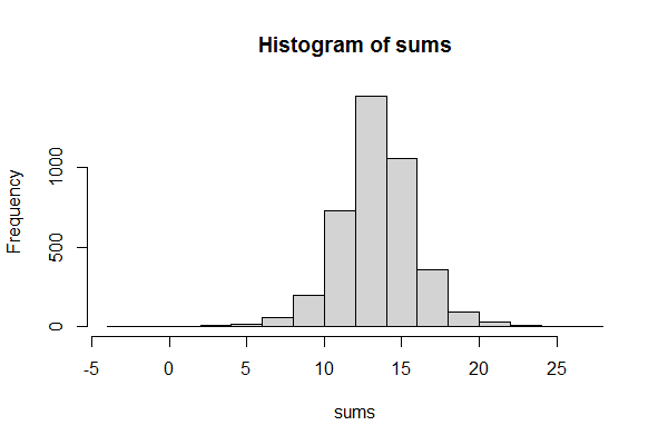
hist(sums)
summary(sums)

So for each regression line in the posterior we computed the predicted values and get a distribution of these values.

enter image description here

$\endgroup$
0
$\begingroup$

I do not know why day is negative in your data and not in sequence from 1, 2, ... I guess those values are obtained after transformation.

For simplicity, assume that we are day in whole number sequence. Suppose that you want to compute $sum(y)$ up to day 10, i.e., $sum_{y10}=y_1 + y_2 + ... + y_{10}$. You need to know $y_8$, $y_9$, and $y_10$. By inserting $y_8=dnorm(a + b * 8, \sigma)$ into your code, you obtain $y_8$. Similarly for the others. Finally you sum $y$ from 1 to 10.

You can insert a for loop when you want to compute for $n$ in general.

Alternatively, you can analytically derive the distribution of $sum(y)$ up to day $n$ using properties of expectation and variance. Note that, $y_1$ to $y_7$ are constant. For example: $$E(sum_{y10}) = y_1 + ... + y_7 + (a+b*8) + ... + (a+b*10)$$ and $$Var(sum_{y10}) = Var(y_8) + ... + Var(y_10) = 3\sigma^2.$$ By this you can monitor $sum_{y10}$ as $dnorm(E(sum_{y10}), 3\sigma^2)$ (or $\sqrt{3\sigma^2}$ if it uses sd instead of var).

Note: The procedure is extrapolation, the result should be used with caution.

$\endgroup$
2
  • $\begingroup$ You're right, days are already transformed. So your solution suggests that I can simulate sum(y) where y>7 and check the final distribution. Am I correct? $\endgroup$ Commented Jan 18, 2021 at 11:43
  • $\begingroup$ Yes, you can generate (or sample) from its posterior distribution by inserting it into the code and monitor it when sampling. $\endgroup$
    – TrungDung
    Commented Jan 18, 2021 at 12:53

Your Answer

By clicking “Post Your Answer”, you agree to our terms of service and acknowledge you have read our privacy policy.

Not the answer you're looking for? Browse other questions tagged or ask your own question.