R: Plot of the relationship between lambda values and coefficients in ridge regression

Question

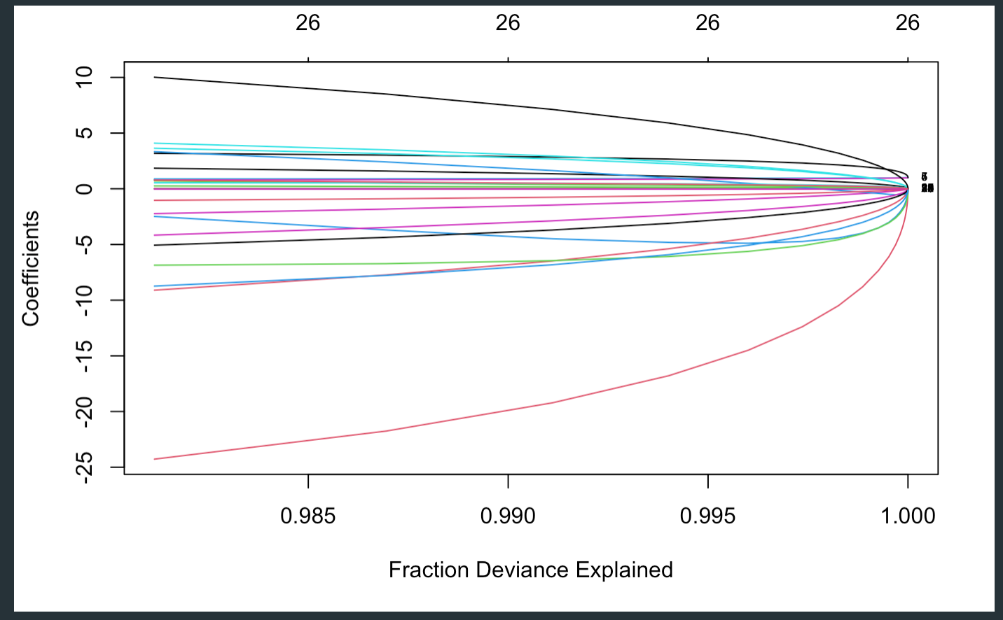
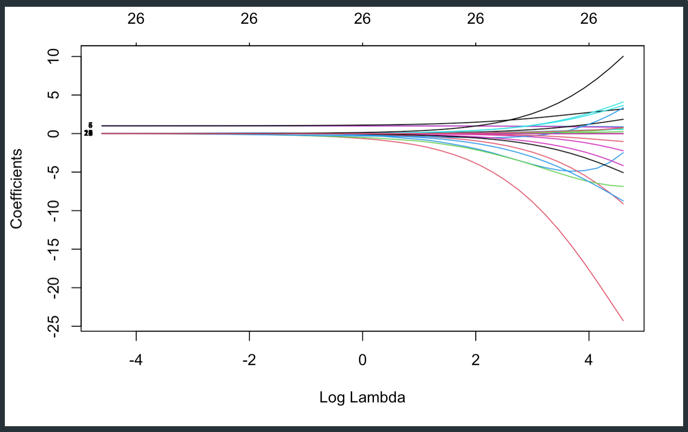
I'm using the code below to plot the relationship between the lambda values used of ridge regression and the coefficients:

lambda_array <- 10^seq(2, -2, by = -.1)

ridge_reg <- glmnet(X_train, 
                   y_train, 
                   alpha=0,
                   lambda=lambda_array)

plot(ridge_reg, xvar = "lambda", label=T)

However, I am getting an unfamiliar output as shown in the image above. This looks like what I would get when plotting the goodness of fit instead. For that I apply:

plot(ridge_reg, xvar="dev", label=T)

Which also gives an unfamiliar output:

I am clueless about what might be happening here.

Some information about the dataset:

• contains several categorical values which were encoded using the ordinal method.
• data was split into testing and training sets which were scaled and converted into matrices in order to use glmnet.
• The values for RMSE, Rsquared and adjustedRsquared (for the optimal lambda of 0.01) are:

[1] 0.2586564
[1] 0.9999986
[1] 0.9999986

The code to compute the values above is:

# y_actual = y_test
# y_predicted = y_pred
rss <- sum((y_pred - y_test)^2)
tss <- sum((y_test - mean(y_test))^2)

# RMSE
RMSE <- sqrt(rss/nrow(df_encoded))
RMSE

# R squared
r_squared <- 1 - (rss/tss)
r_squared

# Adjusted R-squared
adj_r_squared <- 1 - ( ( (1-r_squared)*(nrow(df_encoded)) )  / ( nrow(df_encoded)-ncol(X_train)-1 ) )
adj_r_squared

I was wondering if someone could please explain to me what might be happening here.