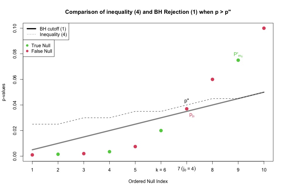
Let's backup and give more context to the two cases specified by equation (5), and then clarify the reasoning behind some of the details.
In equation (5), we consider the two cases, $p \leq p''$ and $ p > p''$
1. $P'_{m_0} =p\leq p''$
This is a difficult (rare) case because all the $m_0$ p-values associated with true nulls are small, and they are likely mixed with false nulls that also have small p-values. By definition of $P'_{m_0} = p \leq p''$, all the true hypotheses (along with $j_0$ false ones) will get rejected by the procedure and we make the maximum error among those $m_0$ true hypotheses. The saving grace is that hopefully $m_0$ is small, or it's very rare (that many Unif(0,1) variables would be smaller than those p-values associated with truly false variables).
"Thus all $m_0 + j_0$ hypotheses are rejected"—why is that? By which procedure? Procedure (1) (=BH)? Or by using the cutoff declared earlier?
Under $p\leq p''$, procedure BH(1) and inequality (4) are effectively describing the same procedure when we consider all true and false hypotheses. It might help to think of the RHS of (4) $:= p''$ as an upper bound on the cutoff described in procedure BH(1) where we think about the index $i$ as $m_0 + j$. Note that at $P'_{m_0}$, the RHS of (1) and (4) are equal, and the $k$ from BH (1) will be $k = m_0 + j_0$ because the maximum of all the true hypotheses are also below this threshold $p''$. I believe the main reason to introduce the inequality like this is for the proof to go through, with the intuition that controlling FDR is limited by the unknown proportion of our tests that are actually true $\left(\frac{m_0}{m}\right)$.
2. $P'_{m_0} = p > p''$
This case is more interesting (common) since our true null p-values are not completely mixed with the false null p-values. Since the true null p-values $P'_{i} \sim Unif(0,1)$, we expect many to fall well above the threshold of rejection (well, at least one, the maximum $P'_{m_0}$), but the goal is to quantify the extent that this happens, which is where we use the induction hypothesis (IH). I think the cleverness here, is that by conditioning out the highest true null p-value $P'_{m_0}$, we can create "new" p-values for a sub-problem with $m$ p-values to allow use of the IH.

I have no idea how they arrive that there must be a k such that $i \leq k \leq m_0 + j - 1$ for which $p_{(k)} \leq \{k / (m+1)\}q^*$ —what is that $j$? Why $−1$?
Under the condition $P'_{m_0} = p > p''$, we are certain that at least 1 value will not be rejected, the hypothesis associated with $P'_{m_0}$. Again, it's useful to think of $p''$ as an upper bound on the cutoff provided by BH (1). Even though these cutoff values for inequality (4) are defined on only the false nulls, no matter how $P'_{m_0}$ lands among the false p-values, $P'_{m_0} > p''$ exceeds the upper bound of the rejected p-values of the BH condition always since the upper bound of (4) does not change for true null p-values (in the plot, dashed line only inflects upwards on false nulls).
The $j$ here is the same $j$ preceding equation (4). The "$-1$" is here because we're creating a sub-problem by conditioning on the maximum true null p-value. The maximum value of $j$ is $m_1$, so the largest our sub-problem is $m_0 + m_1 - 1 = m$.
We create the associated sub-problem by creating new Unif(0,1) random variables dividing by the maximum $p$, and it happens that the new selection problem has $m_0 + j - 1$ p-values, associated with the constant $\frac{m_0 + j - 1}{(m+1)p}q^*$.
From here, the proof is largely algebraic, and it seems you understand the remaining portions.
For completeness and the curious, associated code for the plot is below!
qs <- .05 # FDR control rate
m0 <- 4 # num true H0
m1 <- 6 # num false H0
ix <- 1:10 # Index of all true/false H0
jx <- c(1, 1, 2, 2, 3, 3, 4, 5, 5, 6) # Index increases when H0 false
pval <- c(.001, .0015, .002, .0035, .0075, .02, .037, .06, .075, .1)
plot(ix, pval,
     xlim = c(1, 10),
     ylim = c(0, .1),
     col = c(2, 3, 2, 3, 2, 3, 2, 2, 3, 2),
     cex = 1.5,
     pch = 19,
     xlab = "Ordered Null Index",
     ylab = "p-values",
     xaxt = "n")
title(main =
  'Comparison of inequality (4) and BH Rejection (1) when p > p"')
lines(ix, ix / 10 * qs, col = rgb(0,0,0, alpha = .5), lwd = 4) # BH cutoff
lines(ix, (m0 + jx) / (m0 + m1) * qs, lty=2) # (4) RHS

# Various labels and legends
text(9, .075, expression("P'"[m[0]]), pos = 3, cex = 1.1, col = 3)
text(7.2, .0355, expression("p"[j[0]]), pos = 1, cex = 1.1, col = 2)
text(7, .04, 'p"', pos = 3, cex = 1.1)
axis(1, at = 1:10, labels = c("1", "2", "3", "4", "5", "k = 6",
    expression(7 ~ (j[0] ~"="~ 4)), "8", "9", "10"))
legend("topleft", lty = c(1, 3), lwd = c(4, 1),
    legend = c("BH cutoff (1)", "Inequality (4)"))
legend(x = .64, y = .0909, col = c(3, 2), pch= c(19, 19),
    legend = c("True Null", "False Null"))

