What are the rules on when it is acceptable to use a paired t-test?

Question

I'd appreciate some help understanding exactly where the boundary lies between experiments where a paired t-test can be used, versus an independent t-test.

The simple examples I've found online make sense. A paired t-test might be useful to see if a set of lab rats were affected by a stimulus. For the same set of lab rats, we can measure their brain activity before and after the stimulus and test the significance with a paired t-test.

If I'm unable to do a before and after from the same set of lab rats, but instead the unstimulated lab rats are disjoint from the stimulated lab rats, I have to run the independent t-test. Intuitively, we have to account for the typical deviation in brain activity among a sample of lab rats.

But to torture the analogy, suppose I have the genetic code for N different lab rats, and I clone 2 rats from each genetic code and raise them for a few weeks. For each genetic code sample, one of the pair of cloned rats goes into the control sample, the other into the test sample. So I have two sets of size N. I stimulate a test sample of size N. And I leave the control sample of size N alone.

Is this an appropriate use of a paired test? I could argue yes - each pair comes from the same genetic code. But I could also argue no - although each pair comes from the same genetic code, each pair has had lots of other noisy events in their lives that adds noise.

Answer 1

Independent two-sample data. Two sample t tests (pooled or Welch) are appropriate for samples drawn independently from two different normal (or nearly normal) populations. Samples need not be of the same size. Welch t test should be the default, unless you have good reason to believe the two populations have the same variance.

Examples, using fictitious data sampled in R:

set.seed(616)
x1 = rnorm(40, 100, 15)
x2 = rnorm(50, 103, 17)

summary(x1);  length(x1);  sd(x1)
   Min. 1st Qu.  Median    Mean 3rd Qu.    Max. 
  58.75   92.29  103.84  101.93  112.42  136.61 
[1] 40        # sample size
[1] 13.98087  # sample SD

summary(x2);  length(x2);  sd(x2)
   Min. 1st Qu.  Median    Mean 3rd Qu.    Max. 
  54.76   91.12  100.52  100.77  113.98  134.66 
[1] 50
[1] 16.66023

Population means $\mu_1 = 100, \mu_2 = 103$ differ, but on account of the variability, sample means $\bar X_1 = 101.93, \bar X_2 = 100.77$ do not differ significantly (and, in this particular situation, are in the reverse order).

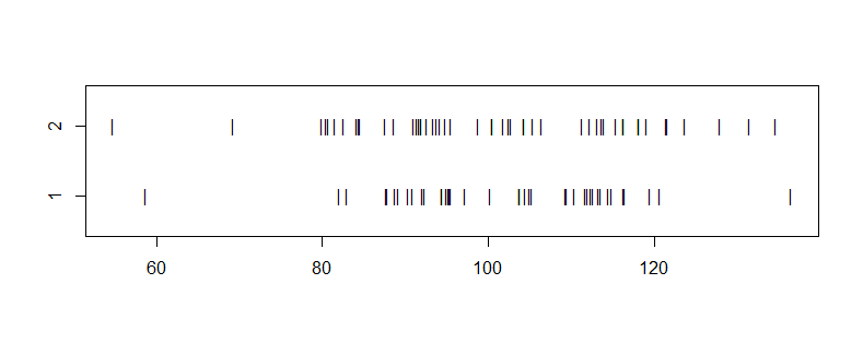
Stripcharts show how variability obscures the difference in location.

stripchart(list(x1,x2), ylim=c(.5,2.5), pch="|")

Also, the P-value $0.722 > 0.05 = 5\%$ shows there is no significant difference between population means at the 5% level.

t.test(x1,x2)

        Welch Two Sample t-test

data:  x1 and x2
t = 0.35689, df = 87.778, p-value = 0.722
alternative hypothesis: 
 true difference in means is not equal to 0
95 percent confidence interval:
 -5.267667  7.573743
sample estimates:
mean of x mean of y 
  101.927   100.774 

If the two sample sizes happen to be equal (the most efficient use of a given number of subjects), one could see if the sample correlation $r$ happens to be far from $0.$ Typically, this will not occur, because the samples are taken independently from different populations.

set.seed(617)
w1 = rnorm(35, 100, 15)
w2 = rnorm(35, 103, 16)
mean(w1); mean(w2)
[1] 97.60775
[1] 104.3471
cor(w1,w2)
[1] -0.06332809

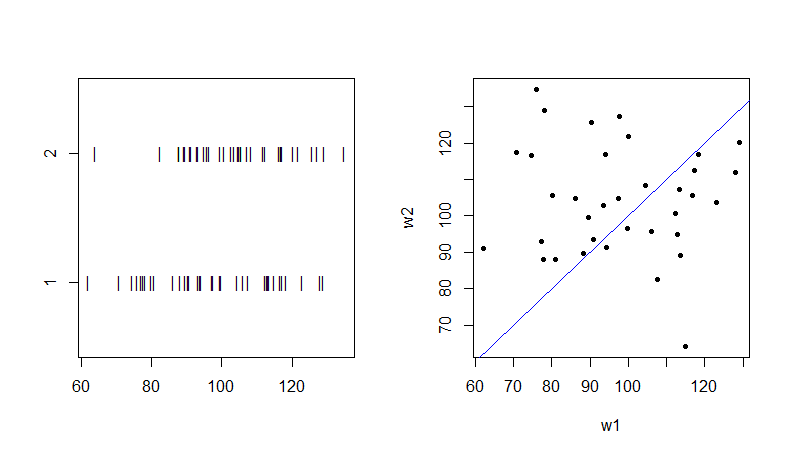
The population means differ, as before, but the difference between them is not statistically significant at the 5% level. Also, $r \approx 0$ and a chaotic scatterplot indicate there is no (chance) association between the two samples.

par(mfrow=c(1,2))
 stripchart(list(w1,w2), ylim=c(.5,2.5), pch="|")
 plot(w1, w2, pch=20);  abline(a=0,b=1,col="blue")
par(mfrow=c(1,1))

Again here, a Welch 2-sample t test has a relatively large P-value, indicating no significant difference between the two sample means at the 5% level.

t.test(w1,w2)$p.val
[1] 0.08918601

Paired data. You have one sample of $n$ pairs from a possibly variable population. A 'pair' may be two observations (e.g., Before and After) on a single individuals. Or it may be observations on two 'similar' subjects (e.g., twins or carefully matched for age, weight, gender, ethnicity, disease status, or other relevant factors.)

Ultimately we are interested in the difference $d_j = Y_{2,j} - Y_{1,j}$ between the two observations in each pair $j = 1, 2, \dots, n.$ Values $d_j$ may be positive or negative, but for paired t tests they are assumed to be normally distributed. Observations (test scores, lab tests, etc.) may be subject to their own variability, which one hopes is smaller than the variability among pairs.

Our data may first appear as $y_{1j},$ and $y_{2j} = y_{1j}+ d_j,$ but it is the differences $d_j$ that matter. If we put data y1, y2 into a paired test procedure, the first step is to find differences d.

set.seed(618)
d = rnorm(35, 3, 1)
summary(d);  length(d); sd(d)
   Min. 1st Qu.  Median    Mean 3rd Qu.    Max. 
 0.3012  2.3025  3.0661  2.8160  3.3869  5.0838 
[1] 35
[1] 1.068237

y1 = rnorm(35, 100, 15)
y2 = y1 + d
cor(y1, y2)
[1] 0.9971784

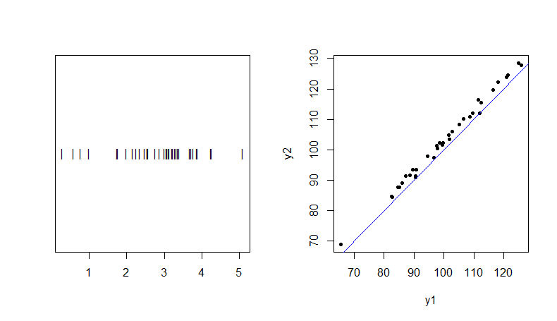
If you look at y1, y2, you will typically see that they are highly correlated. If the $d_i$ have a mean significantly different from $0,$ then points on a scatterplot tend to lie mostly on one side of the 45-degree line.

par(mfrow=c(1,2))
 stripchart(d, pch="|")
 plot(y1, y2, pch=20); abline(a=0,b=1,col="blue")
par(mfrow=c(1,1))

par(mfrow=c(1,2))
 stripchart(d, pch="|")
 plot(y1, y2, pch=20)
  abline(a=0,b=1,col="blue")
 par(mfrow=c(1,1))

A paired test for these fictitious data shown significance. We illustrate that the paired t test is the same as a one-sample t test of the differences.

t.test(y2,y1, pair=T)

        Paired t-test

data:  y2 and y1
t = 15.595, df = 34, p-value < 2.2e-16
alternative hypothesis: 
 true difference in means is not equal to 0
95 percent confidence interval:
 2.449033 3.182937
sample estimates:
mean of the differences 
               2.815985 

t.test(d)

        One Sample t-test

data:  d
t = 15.595, df = 34, p-value < 2.2e-16
alternative hypothesis: 
 true mean is not equal to 0
95 percent confidence interval:
 2.449033 3.182937
sample estimates:
mean of x 
 2.815985 

Answer 2

It all comes down to having a reasonable experimental design for your particular domain. Ideally, paired data points should have absolutely everything the same except for the factor you're studying. We typically design paired experiments to maximize that similarity, but it's never truly the case. Take your classic Before/After paired study for example. A good experiment will control as many "pertinent" factors as possible, leaving only the intervention under study as the difference between Before and After. But even though you can control lots of explicit things, there will still be differences in Before and After that you haven't accounted for - maybe a cosmic ray introduced some DNA mutation, or changing barometric pressure introduces some effect, or any number of other factors you haven't accounted for.

The best you can do is try to achieve as much similarity as possible between your paired samples, but there is no hard line where samples are "sufficiently similar" to count as paired. Something that counts as "sufficiently similar" in one context may not be in another. If you're studying effects that are entirely determined by genetics alone, having two mice of identical genetic code is probably sufficient to count as paired. But if you're running an experiment to investigate effects that have nothing to do with genetics, pairing based on genetics won't indicate any kind of meaningful similarity by which to pair samples.

Answer 3

I think the answer to your question follows much more naturally from the answer to the related question: what are the rules on when it is acceptable to use an unpaired t-test? The first (and least up for negotiation) assumption is that the data are independent. (Along with checking the other assumptions about the error term.)

If this independence assumption doesn't hold, whether this is because it was the same animal at two time points, because the animals were clones, or even because they were litter mates or were housed together, this particular assumption is violated and you shouldn't use an independent sample t-test without having a particular justification for why the data are (at least for all intents and purposes) independent.

There are many ways you could accommodate non-independence in your data, including random effects and GEEs, and with versions of some statistical models such as MANOVA, RM-ANOVA, Friedman's test, etc.

One of the options is to turn the non-independent data into independent summary measures, which is what a paired t-test does. All a paired t-test is is a one-sample t-test on the differences between pairs. As such the assumptions for this test (assuming you are interested in the p-value and not just the effect size) are that the differences are sufficiently normally distributed (given the sample size) for the central limit theorem to come into play and that the differences themselves are independent. If the differences are not sufficiently normally distributed, you might consider a Wilcoxon signed-rank test, for example.

It's not a matter of your data being sufficiently paired to justify a paired t-test, it's a question of whether your data are independent and so can be analysed (subject to the other assumptions involved) using an independent sample t-test. If the data are not independent, you'll need to decide how to accommodate this, with a paired t-test being one of the potential approaches.