How to determine long-term coexistence in a stochastic simulation?

Question

I wrote a stochastic simulation to investigate a system in which replicators proliferate in compartments (rudimentary cells). The compartments contain two kinds of replicators: master sequences and mutants. Mutants can drive the system into extinction. I'm interested in where coexistence is possible in the parameter space.

The Model

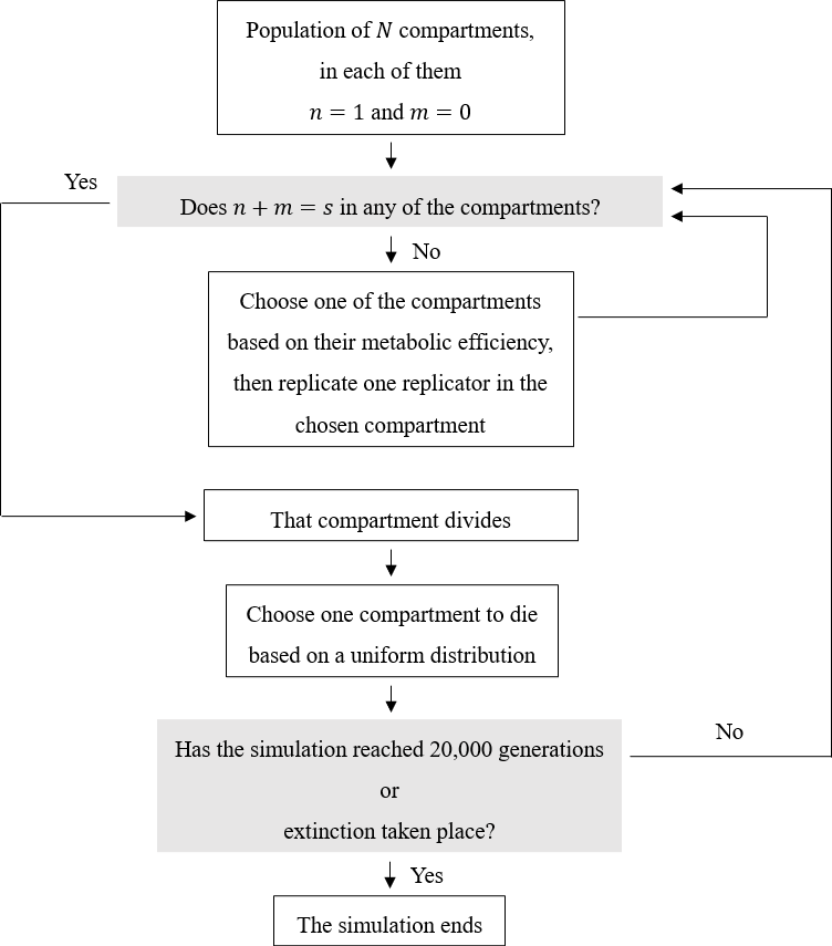
The link above points to a version with non-overlapping generations, but these systems are usually modelled with overlapping generations. The following image is the flow diagram of the model with overlapping generations.

$N$ is the compartment population size, $n$ is the number of master sequences in a given compartment, and $m$ is the number of mutants in a given compartment, $s$ is split size (the total number of replicators in a compartment at which the compartment divides).
The metabolic efficiency of a compartment is the number of master sequences it harbours divided by the total number of master sequences in the system.
Replication happens by randomly choosing a replicator based on replication rates. If a master sequence is chosen to replicate, it mutates to a mutant with probability $U$.
You can read about compartment division here.
One generation corresponds to $N$ compartment divisions.
The population counts as extinct when there are no master sequences left in any compartment.

My aim

With a given $(N,s,\text{relative mutant replication rate})$ combination, I search for the highest value of the mutation rate, with two decimal place accuracy, at which the population survives, i.e. master sequences and mutants coexist.
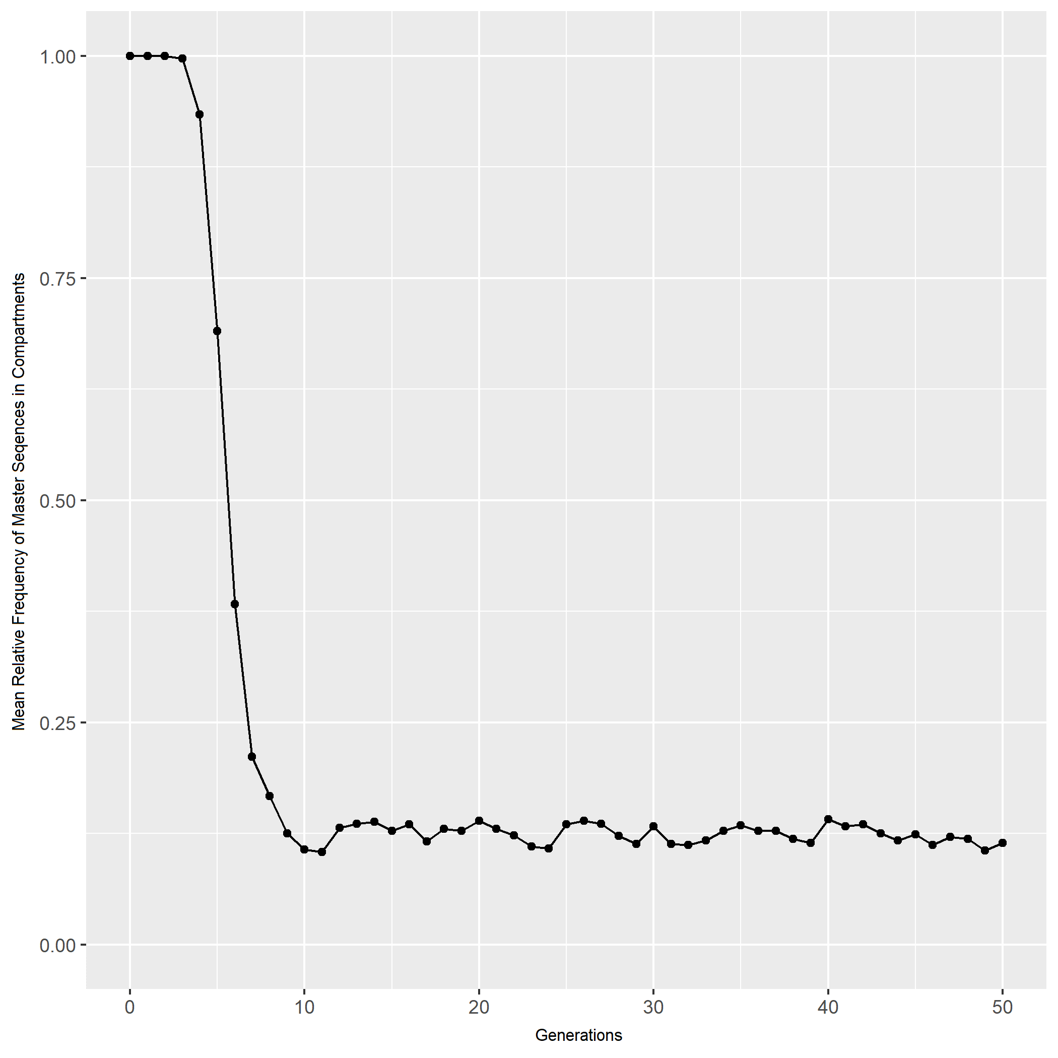
Coexistence does look different from extinction. It looks like an equilibrium:

But I'm reluctant to call it an equilibrium because this is a stochastic model with one absorbing state, so as far as I know, the mutant will eventually fix with probability $1$.

How to determine what counts as coexistence?

It is usually done by choosing a maximal number of generations. This choice is primarily constrained by the available computing power and time.
For example, I have done preliminary simulations of the above system with an insane amount of maximal generations. It turned out that the majority of extinctions happens before $20000$ generations. And the appearance of time series figures like the above seemed, uh, pretty equilibrium-like in the cases when the system has reached $20000$ generations. So I decided to regard it as coexistence when the system has reached $20000$ generations.
But this seems quite subjective and imprecise. There must be a better way to determine coexistence than guessing it based on figures. Note that I don't want to determine when the system will never go extinct because I actually think it will eventually certainly go extinct (see above). I want to distinguish somehow quick extinction from coexistence during runtime.

I have heard that some do it by fitting a line to the values of a relevant variable (e.g. the number of master sequences in the system) along the generations. They regard it as coexistence and stop the simulation when the slope of this line ceases to be significantly different from zero.
But how should that work? This seems very suspicious to me, raising questions about stopping rules and multiple testing.
Indeed, someone I asked about this said that I shouldn't use significance testing for this. They suggested that I should examine the confidence interval of the slope instead and regard it as coexistence when there are only irrelevant values in the confidence interval. But then, how is that more objective?

Questions

So what is a proper, statistically sound way to do this? What are the relevant search terms of this topic of determining the "equilibrium" of a system like this?

Answer 1

The concept you need is the “quasistationary distribution”. In systems like this, when the population size is large enough, there exists a quasistationary (metastable, quasiequilibrium) state that will persist almost surely for an exponentially long time compared to that of any initial transient dynamics, exactly as in the figure you’ve shown. Yes, the system will hit zero, but it may sit in quasi-equilibrium until the heat death of the universe…

I don’t know an elementary discussion of the proofs behind the concept, but perhaps this paper by van Doorn and Pollett will be useful: https://www.sciencedirect.com/science/article/pii/S0377221713000799. The intuition for why this state exists has to do with the law of large numbers. When the population size is big enough and the deterministic (N->infinity) limit has a non-zero equilibrium, at finite N, you will have to wait a very long time to get w fluctuation big enough to move the system from “near equilibrium” to “near zero.” Since fluctuation size typically scales like sqrt(N) but distance from quasi-equilibrium to zero scales like N, getting close to zero gets rarer and rarer as N goes up.

As for a simulation procedure to estimate the quasistationary state, the key thing is the quasistationary state is metastable for exponentially longer than the original transient. The theory supports the separation of timescales you see. Run a simulation, wait until it’s good and settled down, and read off the quasi-equilibrium from the trace. If your system has a quasistationary state, the answer will be the same across a huge range of stopping times. If the answer is sensitive to when you stop the simulation, then you do not have a quasistationary state.

A good example working through when the quasistationary state exists is this derivation by Nasell of the “critical community size” for an epidemiological model https://www.cambridge.org/core/journals/advances-in-applied-probability/article/abs/quasistationary-distribution-of-the-closed-endemic-sis-model/C2EAD1B7436261EC9336216592D2C31A.