Modelling conditional coefficient of variation

Question

Suppose we have 10,000 test tubes containing variable concentrations of some chemical. The aim is to use measurements of their chemical contents to characterise the measurement imprecision of a chemical analysis.

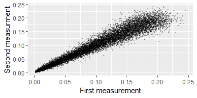
Each test tube is measured twice, and we find the following distribution of first vs. second measurment:

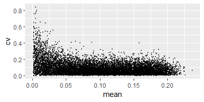
For each test tube we calculate the mean, SD and CV of the pairs of measurements, and observe the following relationship between mean and CV:

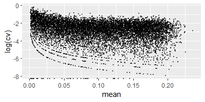
With log(CV) on the y-axis:

(The curve-like pattern in the lower end of the distribution is due to rounding the chemical concentrations two four decimals, which is why CV is also be measured to zero in some instances.)

Obviously, CV is not constant; it is much higher when chemical concentrations are low. I am not interested in trying to estimate a single value of CV that covers all concentrations. Rather, my question is: how can I create a model that predicts the conditional $CV_i$ for any concentration $x_i$ in the range?

EDIT:

First: the reason why I want to do this. Let's say, in the future, the laboratory makes measurement of three independent test tubes and detect concentrations of e.g. 0.0040, 0.0200 and 0.0500. I want to be able to say: for those concentrations, CV is 26.0%, 18.0% and 11.7%, respectively. This means that the 95% CI's for the true concentrations in the test tubes are (0.0021, 0.0060), (0.0129, 0.0271) and (0.0385, 0.0615), respectively.

It would not be a good enough to assume a single, constant CV for all concentrations, as that would make the 95 % CI's incorrect.

Second: the data presented here were simulated. I'm working with real data (about 17,000 paired measurements) that I can't publish here, so I tried to simulate data that would appear somewhat similar. The code used to generate it may not accurately reflect the generating mechanism behind the real data.

I am not a chemical engineer, so I don't know the chemical/physical/technical reason why CV becomes greater when concentrations are lower. However, a chemical engineer explained to me that it is typical: for most of the concentration range, CV tends to be relatively stable, but as you approach the lowest concentrations it increases steeply. This article states this to be true, although it doesn't explain exactly why. Could it simply be mathematical, i.e. that CV tends to increase rapidly as the mean approaches zero? Or maybe lower concentrations are more sensitive to physical/chemical factors influencing the analytical instrument.

Anyway, here is the code:

library(matrixStats)
library(ggplot2)

# Number of simulations
N <- 10000 

# Mu and sigma of the generating process
mu_sim <- runif(N, .002, .2)
sigma_sim <- (.09 + .2 * exp(-40 * mu_sim)) * mu_sim

# Simulate pairs of measurments
data <- data.frame(x1 = round(rnorm(N, mu_sim, sigma_sim), 4),
                         x2 = round(rnorm(N, mu_sim, sigma_sim), 4))

# Calculate mean, SD and CV for each pair
data$mean <- rowMeans(data)
data$sd <- rowSds(as.matrix(data[, 1:2]))
data$cv <- data$sd / data$mean

# Plot of first vs. second measurment
ggplot(data, aes(x = x1, y = x2)) +
    geom_point(size = .5, alpha = .25) +
    labs(x = "First measurement", y = "Second measurment")

# Plot of log(cv) vs. mean 
ggplot(data, aes(x = mean, y = log(cv))) +
    geom_point(size = .5, alpha = .5)

To achieve the effect of rapidly increasing CV towards the lower concentrations and a relatively stable CV for the rest, I used a negative exponential function that quickly declines to a "baseline" CV of 9 % (this number was arbitrarily chosen).

The same article suggests the reciprocal of the variance to be a better measurment of imprecision. However, in this dataset the reciprocal of the variance tends to yield some extremely high numbers, so I don't see how that is of any help.

I would greatly appreciate any help with this problem!

Answer 1

If you create a Bayesian model for the standard deviation, you can do this quite easily.

Let's start with some assumptions. Let draw $i$ from tube $j$ be modelled as

$$ x_{i, j} \sim \mathcal{N}(\mu_j, \sigma(\mu_j)) \>. $$

Here, $\sigma$ is an unknown function of the true concentration. As the true concentration changes, so too does the standard deviation. Note that since we are using a normal distribution, some convenient stuff happens. Namely

• $\mu_j$ can be estimated by the arithmetic mean of the $x_{i,j}$, and
• if $r_j = x_{1, j} - x_{2, j}$ is the residual then $E(x_{1, j} - x_{2, j}) = 0$ and $r_j \sim \mathcal{N}(0, \sigma(\mu_j))$.

So here is what I propose. Let's model the residual as coming from $\mathcal{N}(0, \sigma(\mu_j))$. Once we estimate $\sigma(\mu_j)$ we can easily compute the CV as a function of the latent concentration.

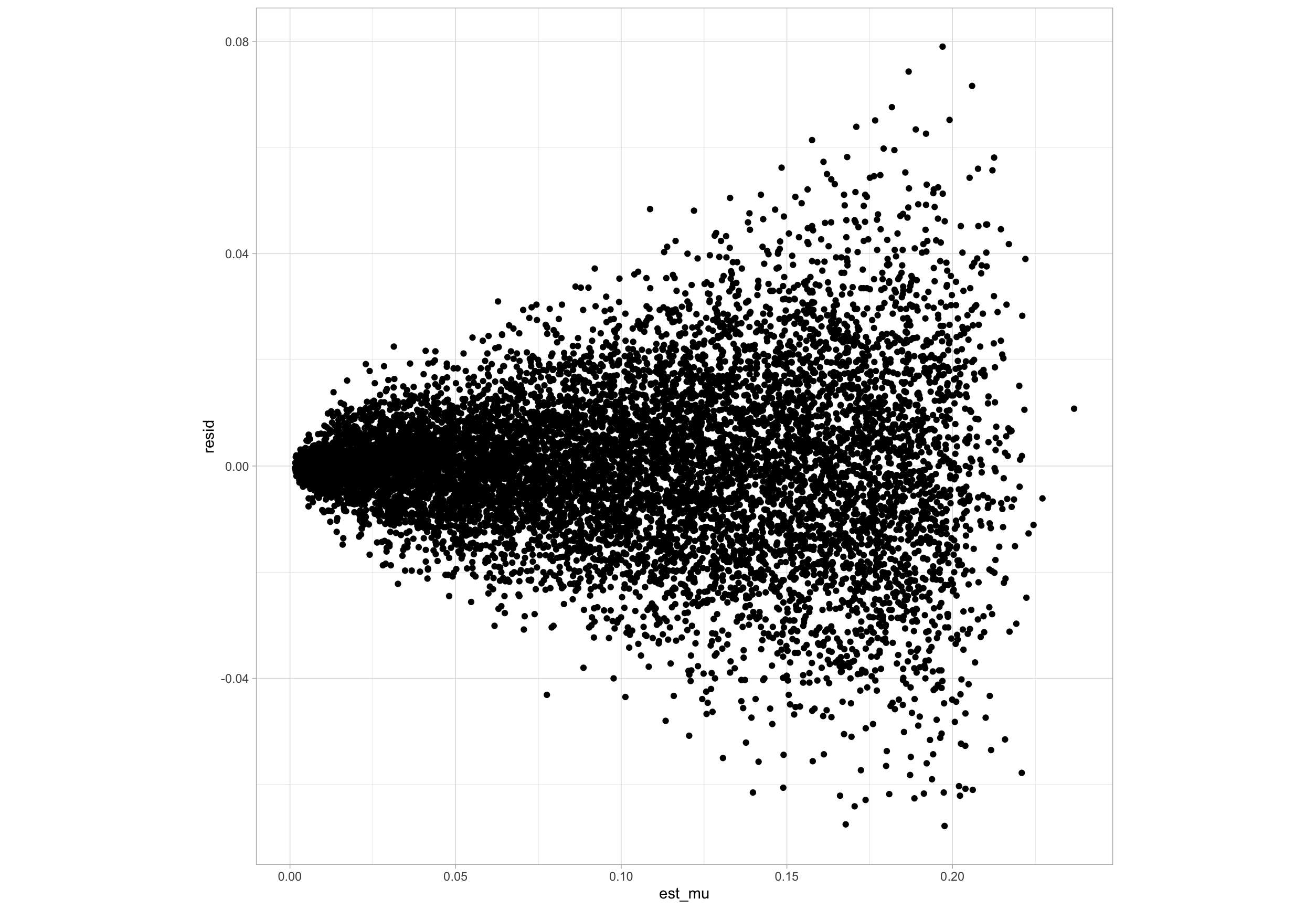
Let's begin with simulating your data and plotting out the residuals versus the estimated mean.

library(tidyverse)
library(tidybayes)
library(cmdstanr)

# Number of simulations
N <- 10000 

# Mu and sigma of the generating process
mu_sim <- runif(N, .002, .2)
sigma_sim <- (.09 + .2 * exp(-40 * mu_sim)) * mu_sim

# Simulate pairs of measurments
data <- tibble(x1 = round(rnorm(N, mu_sim, sigma_sim), 4),
               x2 = round(rnorm(N, mu_sim, sigma_sim), 4)) %>% 
        mutate(resid = x1-x2,
               est_mu = (x1+x2)/2)


data %>% 
  ggplot(aes(est_mu, resid))+
  geom_point()

These data are simulated, but we can see the residuals are evenly distributed around 0 with a variance that changes as the estimated true concentration changes.

Now, we'll write a Bayesian model to estimate the $\sigma(\mu_j)$. There are a lot of ways to do this, but I will take a very easy way and consider $\log(\sigma) = \beta_0 + \beta_s \hat{\mu}$. The full model is

$$ r_j \sim \mathcal{N}(0, \sigma(\hat{\mu_j})) $$

$$ \log(\sigma) = \beta_0 + \beta_s \hat{\mu} $$

$$ \beta_0, \beta_1 \sim \mathcal{N}(0, 1)$$

Here is the Stan model

data{
  int n;
  vector[n] resid;
  vector[n] est_mu;
}
parameters{
  real bs0;
  real bs1;
}
model{
  bs0 ~ std_normal();
  bs1 ~ std_normal();
  resid ~ normal(0, exp(bs0 + bs1*est_mu));
}
generated quantities{
  real resid_ppc[n] = normal_rng(0, exp(bs0 + bs1*est_mu));
}

and we can easily fit it. You'll need cmdstanr and tidybayes to run the remainder of the code.

model_code = <stan code above as a string>
file = write_stan_file(model_code)
model = cmdstan_model(file)
model_data = compose_data(data)
fit = model$sample(model_data)

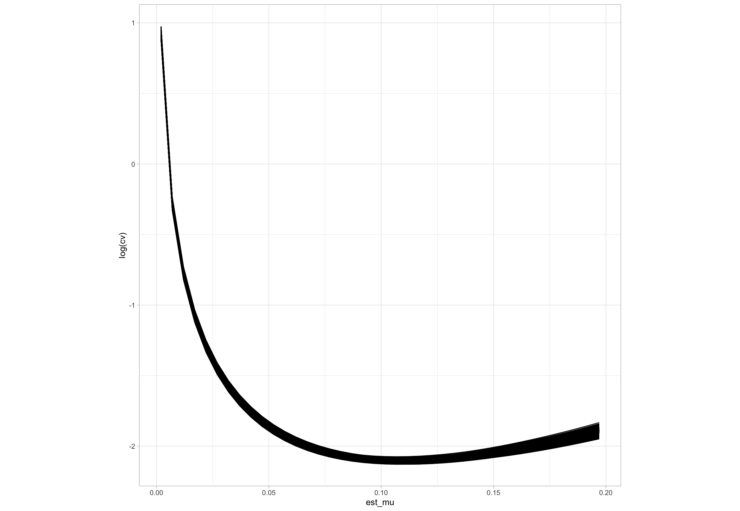
Model runs well. Now, we can use the draws from the model to estimate credible intervals for $cv = \sigma/\hat{\mu}$.

d = tibble(est_mu = seq(0.002, 0.2, 0.005))

fit %>% 
  # Get the draws for the coefficients
  spread_draws(bs0, bs1) %>% 
  # Peform a cross join so that each coefficient pair
  # can create a sigma for each est_mu in d
  left_join(d, by=character()) %>% 
  # create the CV
  mutate(sigma = exp(bs0 + bs1*est_mu),
         cv = sigma/est_mu) %>% 
  # Plot the results, one line per sample
  ggplot(aes(est_mu, log(cv), group = .draw))+
  geom_line()

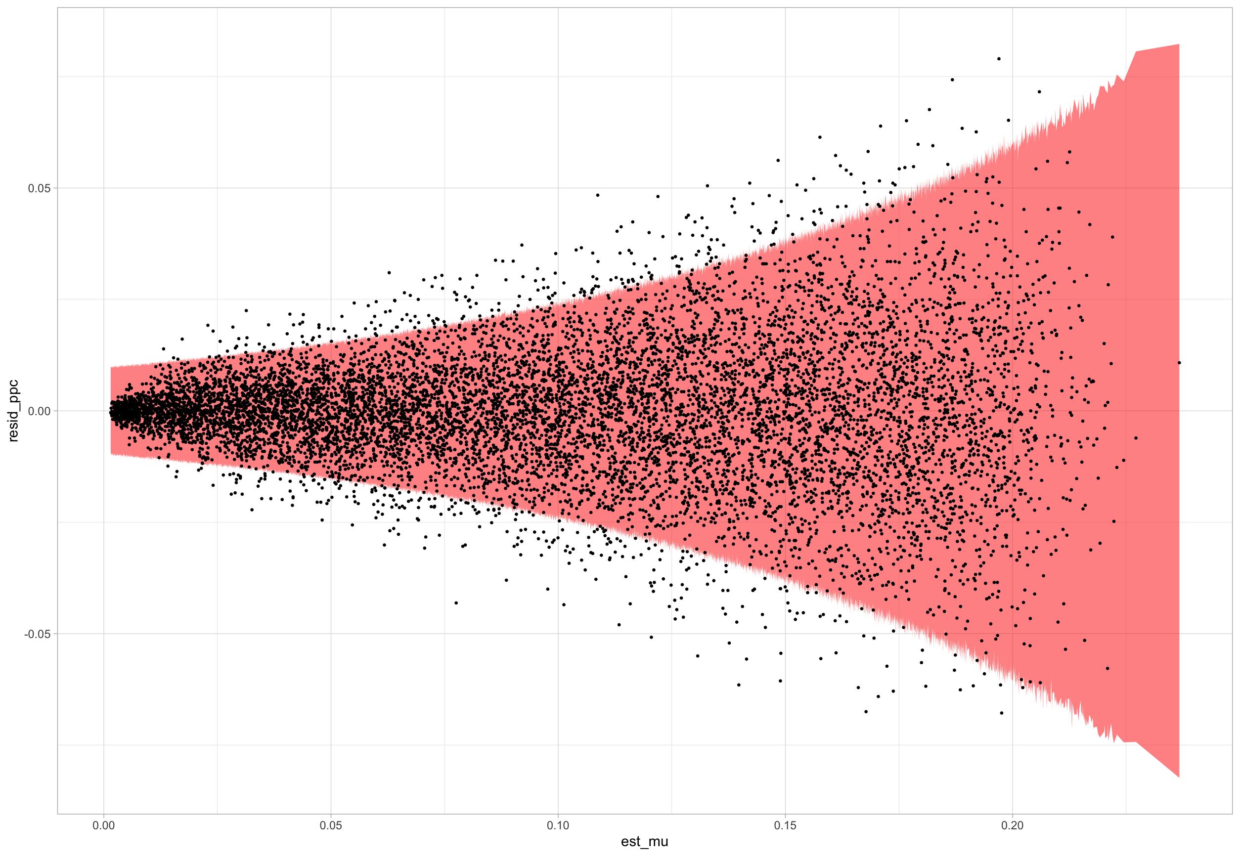
The thick black line is comprised of 4000 individual lines, each considered a draw from the posterior. This doesn't look exactly like your plots, and with good reason -- we didn't use the exact form for the standard deviation you used in your simulation. That is always going to be the case. We can see the extent of the poor fit in this plot. Below I've plotted 95% prediction intervals conditioned on $\hat{mu}$. If the model fit well, then 95% of the black dots would be in the red shaded region. It looks like it might be close, but there is certainly some misfit. The standard deviation is not large enough in most regions, again owing to the fact we misspecified the model (on purpose). You might might want to try using splines rather than modelling the standard deviation as I have, that is if you choose to go this route.