Robust mean estimation with O(1) update efficiency

Question

I am looking for a robust estimation of the mean that has a specific property. I have a set of elements for which I want to calculate this statistic. Then, I add new elements one at a time, and for each additional element I would like to recalculate the statistic (also known as an online algorithm). I would like this update calculation to be fast, preferably O(1), i.e. not dependent on the size of the list.

The usual mean has this property that it can be updated efficiently, but is not robust to outliers. Typical robust estimators of the mean, like inter-quartile mean and trimmed mean cannot be updated efficiently (since they require maintaining a sorted list).

I would appreciate any suggestions for robust statistics that can be calculated/updated efficiently.

Answer 1

You might think of relating your problem to that of the recursive control chart. Such a control chart will evaluate whether a new observation is in control. If it is, this observation is included in the new estimate of the mean and variance (necessary to determine control limits).

Some background on robust, recursive, univariate control charts can be found here. One of the classic texts on quality control and control charts appears to be available online here.

Intuitively, using the a mean, $\mu_{t-1}$ and a variance $\sigma^2_{t-1}$ as inputs, you can determine whether a new observation at time $t$ is an outlier by a number of approaches. One would be to declare $x_t$ an outlier if it is outside of a certain number of standard deviations of $\mu_{t-1}$ (given $\sigma^2_{t-1})$, but this may run into problems if the data does not conform to certain distributional assumptions. If you want to go this road, then supposing you have determined if a new point is not an outlier, and would like to include it in your mean estimate with no special rate of forgetting. Then you can't do better than:

$\mu_t = \frac{t-1}{t}\mu_{t-1}+\frac{1}{t}x_t$

Similarly, you will need to update the variance recursively:

$\sigma^2_t = \frac{t-1}{t}\sigma^2_{t-1}+\frac{1}{t-1}(x_t-\mu_t)^2$

However, you might want to try some more conventional control charts. Other control charts which are more robust to the distribution of the data and can still handle non-stationarity (like the $\mu$ of your process slowly going higher) are the EWMA or CUSUM are recommended (see the textbook linked to above for more details on the charts and their control limits). These methods will typically be less computationally intensive than a robust because they have the advantage of simply needing to compare a single new observation to information derived from non-outlier observations. You can refine your estimates of the long term process $\mu$ and $\sigma^2$ used in the control limit calculations of these methods with the updating formulas given above if you like.

Regarding a chart like the EWMA, which forgets old observations and gives more weight to new ones, if you think that your data is stationary (meaning the parameters of the generating distribution do not change) then there is no need to forget older observations exponentially. You can set the forgetting factor accordingly. However, if you think that it is non-stationarity you will need to select a good value for the forgetting factor (again see the textbook for a way to do this).

I should also mention that before you begin monitoring and adding new observations online, you will need to obtain estimates of $\mu_0$ and $\sigma^2_0$ (the initial parameter values based on a training dataset) that are not influenced by outliers. If you suspect there are outliers in your training data, you can pay the one-time cost of using a robust method to estimate them.

I think an approach along these lines will lead to the fastest updating for your problem.

Answer 2

This solution implements a suggestion made by @Innuo in a comment to the question:

You can maintain a uniformly sampled random subset of size 100 or 1000 from all the data seen thus far. This set and the associated "fences" can be updated in $O(1)$ time.

Once we know how to maintain this subset, we may select any method we like to estimate the mean of a population from such a sample. This is a universal method, making no assumptions whatsoever, that will work with any input stream to within an accuracy that can be predicted using standard statistical sampling formulas. (The accuracy is inversely proportional to the square root of the sample size.)

---

This algorithm accepts as input a stream of data $x(t),$ $t=1, 2, \ldots,$ a sample size $m$, and outputs a stream of samples $s(t)$ each of which represent the population $X(t) = (x(1),x(2), \ldots, x(t))$. Specifically, for $1\le i \le t$, $s(i)$ is a simple random sample of size $m$ from $X(t)$ (without replacement).

For this to happen, it suffices that every $m$-element subset of $\{1,2,\ldots,t\}$ have equal chances of being the indexes of $x$ in $s(t)$. This implies the chance that $x(i),$ $1\le i\lt t,$ is in $s(t)$ equals $m/t$ provided $t \ge m$.

At the beginning we just collect the stream until $m$ elements have been stored. At that point there is only one possible sample, so the probability condition is trivially satisfied.

The algorithm takes over when $t=m+1$. Inductively suppose that $s(t)$ is a simple random sample of $X(t)$ for $t\gt m$. Provisionally set $s(t+1) = s(t)$. Let $U(t+1)$ be a uniform random variable (independent of any previous variables used to construct $s(t)$). If $U(t+1) \le m/(t+1)$ then replace a randomly chosen element of $s$ by $x(t+1)$. That's the entire procedure!

Clearly $x(t+1)$ has probability $m/(t+1)$ of being in $s(t+1)$. Moreover, by the induction hypothesis, $x(i)$ had probability $m/t$ of being in $s(t)$ when $i\le t$. With probability $m/(t+1) \times 1/m$ = $1/(t+1)$ it will have been removed from $s(t+1)$, whence its probability of remaining equals

$$\frac{m}{t}\left(1 - \frac{1}{t+1}\right) = \frac{m}{t+1},$$

exactly as needed. By induction, then, all the inclusion probabilities of the $x(i)$ in the $s(t)$ are correct and it's clear there is no special correlation among those inclusions. That proves the algorithm is correct.

The algorithm efficiency is $O(1)$ because at each stage at most two random numbers are computed and at most one element of an array of $m$ values is replaced. The storage requirement is $O(m)$.

The data structure for this algorithm consists of the sample $s$ together with the index $t$ of the population $X(t)$ that it samples. Initially we take $s = X(m)$ and proceed with the algorithm for $t=m+1, m+2, \ldots.$ Here is an R implementation to update $(s,t)$ with a value $x$ to produce $(s,t+1)$. (The argument n plays the role of $t$ and sample.size is $m$. The index $t$ will be maintained by the caller.)

update <- function(s, x, n, sample.size) {
  if (length(s) < sample.size) {
    s <- c(s, x)
  } else if (runif(1) <= sample.size / n) {
    i <- sample.int(length(s), 1)
    s[i] <- x
  }
  return (s)
}

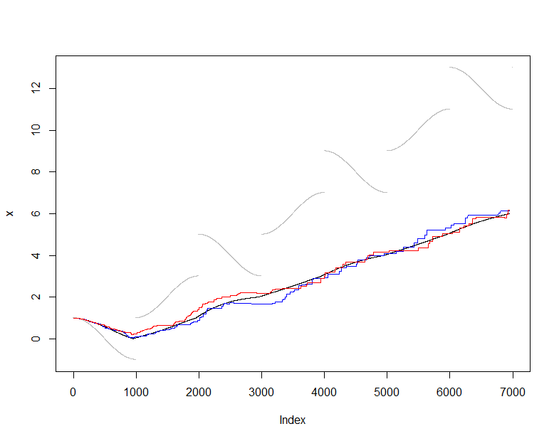
To illustrate and test this, I will use the usual (non-robust) estimator of the mean and compare the mean as estimated from $s(t)$ to the actual mean of $X(t)$ (the cumulative set of data seen at each step). I chose a somewhat difficult input stream that changes quite smoothly but periodically undergoes dramatic jumps. The sample size of $m=50$ is fairly small, allowing us to see sampling fluctuations in these plots.

n <- 10^3
x <- sapply(1:(7*n), function(t) cos(pi*t/n) + 2*floor((1+t)/n))
n.sample <- 50
s <- x[1:(n.sample-1)]
online <- sapply(n.sample:length(x), function(i) {
  s <<- update(s, x[i], i, n.sample)
  summary(s)})
actual <- sapply(n.sample:length(x), function(i) summary(x[1:i]))

At this point online is the sequence of mean estimates produced by maintaining this running sample of $50$ values while actual is the sequence of mean estimates produced from all the data available at each moment. The plot shows the data (in gray), actual (in black), and two independent applications of this sampling procedure (in colors). The agreement is within expected sampling error:

plot(x, pch=".", col="Gray")
lines(1:dim(actual)[2], actual["Mean", ])
lines(1:dim(online)[2], online["Mean", ], col="Red")

---

For robust estimators of the mean, please search our site for outlier and related terms. Among the possibilities worth considering are Winsorized means and M-estimators.