How to interpret a polychoric correlation?

Question

I've checked related links to understand what a Polychoric Correlation measures, got some 404's and other unanswered questions. I've seen it used to determine independence between Nominal/Interval ( "Contunuized"*, aka, Jointly Normal ) on YouTube (https://www.youtube.com/watch?v=besaBez9giw&t=597s), as ways of measure correlation between (underlying continuous ) variables, and I've seen it used to describe the distribution of some (underlying continuous ) trait of fertility of cattle given data on cattle births (From John Uebersax' page ).

I (think I) understand the general underlying setup for the polychoric. We start with a paired discrete/Interval/Ordinal data set . We assume each data set is discrete output comes from an underlying Normal Distribution , and the pair of variables is jointly-normal. The poly/tetra choric is then the Pearson correlation between these underlying continuous variables . Is this correct? If so, does it have / can it be used for the purposes described in the above paragraph?

Edit: Also, are normality of each and joint normality required? How robust is it (i.e., how well does the test fare under departures from normality assumptions). Because doesn't joint normality equivalent to individual Normality?

Answer 1

Let me provide my answer using the tetrachoric correlation (which is the polychoric correlation when you have two dichotomous ordinal variables).

First, the answer to the first question is: "yes"...this would be the correlation of the underlying (i.e., unobserved) latent variables. And, based on the assumption that the last concept is dichotomous/ordinal, the correlation could be applied to describe the hypothetical underlying distribution.

To clarify, for the calculation of our correlation, we are assuming that our dichotomous observations are actually continuous (normally distributed) values...but they have been dichotomized because these fall above/below some cut value ($\tau$). So we observe $x=0$ or $x=1$, but this we are assuming that this is really $x=0$ if $\xi < \tau$ and $x=1$ if $\xi > \tau$...and the "real" data (even if we can't see it) is $\xi$. So, in your example, the underlying fertility trait is $\xi$ and we are just observing the dichotomized $x$. (The terminology from latent variable analysis is that $\xi$ is the latent/unobservable variable and $x$ is the manifest/measured/observed variable.)

Now, if we assume the same thing for our 2nd variable, say $y$ (with an underlying $\eta$ variable), then we call the correlation of $\xi$ and $\eta$ the tetrachoric correlation.

A brief comment on how this is estimated: using the marginal means and the distribution of the values into the four quadrants (cells of the 2×2 contingency table), we can estimate the $\tau$ cuts and the $\rho$ correlation of the latent variables. We often make simplifying assumptions such as the variance of the latent variables are 1...and if we can't actually measure them anyway, the actually degree of spread is kind of arbitrary...so might as well make is easy to work with.

Second brief comment: for ordinal variables, the same idea holds...but now we have more than one $\tau$-cut to subdivide the normal distribution into regions associated with the different values of the ordinal measure.

Now for the next question: ¿do we need to assume that the underlying distributions are normal? Well, the key idea here is that we are attempting to describe something that can never be measured or directly observed. So, we really don't know what the distribution would be. So, to my earlier point, if we can't actually see it, we get some freedom in how we choose to describe it. As such, we can make our life easier by picking a distribution that is relatively easy to work with...so, why not pick the normal distribution.

Another way to think about this is if you place the $\tau$ cuts on a normal distribution, you obtain a set of relative frequencies for each value of the ordinal measure. In truth, if you picked a different distribution, you could obtain those same (marginal) percentages, you just would have to pick your new $\tau$-cuts accordingly.

So, the question of robustness may not be contextually appropriate here. While I believe you could obtain different estimates for the underlying correlations for different distributions, this is a question about when we know specific information about the "latent" variable...but if we really knew that much information about these types of variables, they probably would be observable, and we wouldn't actually need to do a latent analysis.

I hope this helps. Happy to clarify anything as needed.

---

UPDATE #1a
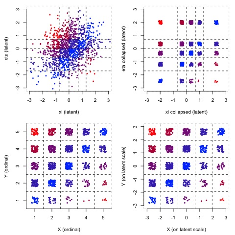
Here is a graphic I generated to help elaborate on this idea.

UPDATE #1b
Here is some brief commentary about the graphic from yesterday. For my personal learning, I have found it very useful to "visualize" the assumptions of the models. As such, I like to think about the actual data generation process that might play out.

In this context, the "assumption" is that the latent variables follow a bivariate normal distribution, and there are some cuts along the latent scale that separate observed data into the ordinal categorical scores. To clarify, I believe the assumption of bivariate normality is just a convenience, as you could obtain any marginal relative frequencies with ANY distribution if you position the tau-cuts appropriately. So, since we can't see what the wizard is really doing behind the curtain, let's just keep it simple since we now how to work with normal distributions.

So, the upper-left graphic shows a simulated draw from a bivariate normal distribution (with N(0,1) for each marginal distribution and a fixed rho of 0.3. I kinda just made up some tau-cuts for each axis and I've color coded to help distinguish distance from the diagonal of rectangles formed by the tau-cuts.

The next graphic simply "collapses" all the observations in each rectangle to one bunch. The idea here is that if we have this pattern of bivariate data with these tau-cuts, these are reasonable relative frequencies to see for a corresponding 5x5 contingency table for our observed ordinal data.

The next graphic (lower-right) just makes the rectangles all the same size, and the last graphic (lower-left) just relabels the observed data in the fashion we would see it.

So, what polychoric correlation is doing is taking this process and trying to run it in reverse. We start with a relative frequency pattern for our contingency table of ordinal data in the lower-left, and we find the optimal solution for correlation and tau-cuts to get us back to a bivariate normal distribution that would have comparable relative joint-frequencies.

Answer 2

The answer by Gregg H is very good. However I'd like to add something about the "assumption" of normality. The whole concept of polychoric correlation is based on the normality assumption. In fact the same observable distribution of categories is compatible with any continuous marginal distribution, and I'm pretty convinced that often the correlation between two latent variables can take a large range of values if we try to find "worst case" non-normal underlying distributions that move the correlation as far away from the one under normality assumption as possible. This is because the correlation is very sensitive to outliers, so that shifting small probabilities to infinity in the latent distribution will have a huge impact on correlations. (Note that for sure the latent distributions can be chosen so that second moments, and therefore correlations, do not exist.)

So statements about the "true" correlation between the "true" latent variables will not be robust, and one can't just justify using the normality assumption for convenience reasons. There is no way to test it either, as Gregg H correctly noted. In fact it is possible to test whether the dependence structure is like a normal one (Gaussian copula), but this is not enough to make sure that correlations are robust, as outliers can spoil the correlation through the marginal distributions even if the dependence structure is fixed.

This seems quite negative, however my own interpretation would be different. I do not think that it is in fact required that the "true" underlying distribution is Gaussian; I'd rather say that the polychoric distribution is a measure of correlation between the observed categorical variables that is "calibrated" through an underlying Gaussian model. The role of the Gaussian model here is not to be "true", but rather to fix a setup that allows to compute a correlation measure. The Gaussian is symmetric and does not have heavy tails, so it will lead to a rather regular and intuitive correlation measure; skew distributions or distributions with outliers will imply correlations that are less intuitively connected to the observed categorical dependence, therefore less desirable. (In fact I believe that the Gaussian correlation will be more robust, at least regarding what happens working with similarly "nice" distributions, than any correlation based on a skew or heavy-tailed distribution, even though worst cases will always be bad).

So there is a way to use polychoric correlations that in my view makes sense regardless of whether there is a "true latent distribution". In most cases I'd say that such a distribution does not really exist, rather it is a modelling device, and then we can choose a nice and convenient one. However, beware of interpreting polychoric correlations as true correlations between real latent variables.