It's useful to know how to convert the notation of Complex numbers into a more familiar Real notation. Here are the details.
Hermitian matrices and real-valued Complex forms
$\mathbf Q = (q_{ij})$ is a square matrix representing a real-valued quadratic form. This means that we don't really care about the details of $\mathbf Q:$ what matters is the function of the (Complex) vector $\mathbf z = (z_1, z_2, \ldots, z_n)^\prime$ defined via matrix multiplication by
$$Q(\mathbf z) = \mathbf z^{*}\, \mathbf Q\, \mathbf z = \sum_{i=1}^n \sum_{j=1}^n \bar z_i\, q_{ij}\, z_j.\tag{1}$$
Writing $z_i = x_i + y_i\mathbf i$ in terms of its real and imaginary parts, the overline refers to the complex conjugate $\bar z = x_i - y_i\mathbf i$ and the conjugate transpose operation transposes a vector and conjugates all its components,
$$\mathbf z^* = (\bar z_1, \bar z_2, \ldots, \bar z_n).$$
Because $Q$ is required to be a real number for all such vectors $\mathbf z,$ it must equal its conjugate, whence (by swapping the symbols "$i$" and "$j$" in the sums) we see
$$Q(\mathbf z) = \overline {Q(\mathbf z)} = \sum_{i=1}^n \sum_{j=1}^n z_i\, \bar q_{ij}\, \bar z_j = \sum_{j=1}^n \sum_{i=1}^n z_j\, \bar q_{ji}\, \bar z_i$$
Comparing this to $(1)$ shows that for equality to hold for all $\mathbf z,$ necessarily $q_{ij} = \bar q_{ji}$ for all indexes $i$ and $j.$ Such a matrix is called Hermitian and this operation of transposing a matrix while taking complex conjugates is evidently a generalization of the conjugate transpose, allowing us to write
$$\mathbf Q^{*} = (\bar q_{ji}) = \overline{\mathbf Q}^{\prime}.$$
In other words,
A Complex quadratic form $Q$ is real if and only if the matrix $\mathbf Q$ representing $Q$ is Hermitian.
Writing Complex forms as equivalent Real forms
Write $q_{ij} = a_{ij} + b_{ij}\mathbf i.$ The Hermitian property of $\mathbf Q$ is
$$a_{ji} - b_{ji}\mathbf i = \bar q_{ji} = q_{ij} = a_{ij} + b_{ij}\mathbf i.$$
Comparing real and imaginary parts and assembling them into matrices $\mathbf A = (a_{ij})$ and $\mathbf B = (b_{ij})$ shows
$$\mathbf A = \mathbf A^\prime\ \text{and}\ \mathbf B = -\mathbf{B}^\prime.\tag{2}$$
$\mathbf A = \Re (\mathbf Q)$ is the real part of $\mathbf Q$ and $\mathbf B = \Im (\mathbf Q)$ is its imaginary part. If these (simple) relationships are not perfectly clear, see the concrete example (with $n=2$) offered at the end of this post.
Let $i$ and $j$ be arbitrary indexes. Let's examine how the real and imaginary parts of $z_i$ and $z_j$ appear in $Q(\mathbf z).$ This product appears in at most two terms in the sum $(1),$ which can be combined using the Hermitian property of $\mathbf Q.$ Here is the calculation when $i\ne j.$ We only have to compute the real part of the result, knowing the imaginary part will be zero.
$$\begin{aligned}
\bar z_iq_{ij}z_j + \bar z_jq_{ji}z_i &= (x_i - y_i\mathbf i)(a_{ij} + b_{ij}\mathbf i)(x_j + y_j\mathbf i) + (x_j - y_j\mathbf i)(a_{ji} + b_{ji}\mathbf i)(x_i + y_i\mathbf i)\\
&= (x_i - y_i\mathbf i)(a_{ij} + b_{ij}\mathbf i)(x_j + y_j\mathbf i) + (x_j - y_j\mathbf i)(a_{ij} - b_{ij}\mathbf i)(x_i + y_i\mathbf i)\\
&= 2x_i\, a_{ij}\, x_j + 2y_i\, a_{ij}\, y_j - 2x_i\, b_{ij}\, y_j + 2 x_j\, b_{ij}\, y_i
\end{aligned}$$
(I leave the calculation for $i=j$ as a simple exercise.)
This is a quadratic form in the $2n$ dimensional real vector $\mathbf z_{\Re} = (x_1,x_2,\ldots, x_n;y_1,y_2,\ldots,y_n).$ In block matrix notation its matrix is
$$\mathbf Q_{\Re} = \pmatrix{\mathbf A & -\mathbf B \\ \mathbf B & \mathbf A}.\tag{3}$$
Because $\mathbf A$ is symmetric and $\mathbf B$ is antisymmetric (according to $(2)$ above), evidently $\mathbf Q_{\Re}$ is a real, symmetric matrix -- as it must be, because we have already seen it represents a real-valued quadratic form in the real variables $x_1, \ldots, y_n.$
Solution to the problem in the question
Our thread at Variance of quadratic form for multivariate normal distribution shows that
$$\operatorname{Var}\left(\mathbf z^* \mathbf Q\, \mathbf z\right) = \operatorname{Var}\left(\mathbf z_{\Re}^\prime\, \mathbf Q_{\Re}\, \mathbf z_{\Re}\right) = 2\operatorname{tr}\left(\mathbf Q_{\Re}^2\right).$$
The block matrix expression for this form's matrix enables us to compute this trace in terms of the real and imaginary parts of $\mathbf Q,$
$$\operatorname{tr}\left(\mathbf Q_{\Re}^2\right) = \operatorname{tr}\left(\pmatrix{\mathbf A & -\mathbf B \\ \mathbf B & \mathbf A}^2\right) = \operatorname{tr}\pmatrix{\mathbf A^2 - \mathbf B^2 & -2\mathbf A \mathbf B\\2\mathbf B \mathbf A & \mathbf A^2 - \mathbf B^2} = 2\operatorname{tr}\left(\mathbf A^2\right) - 2\operatorname{tr}\left(\mathbf B^2\right).$$
Thus,
$$\operatorname{Var}\left(\mathbf z^* \mathbf Q\, \mathbf z\right) = 4\operatorname{tr}\left(\mathbf A^2 - \mathbf B^2\right) = 4\left(\operatorname{tr}\Re(\mathbf Q)^2 - \operatorname{tr}\Im(\mathbf Q)^2\right).$$
Checking the result
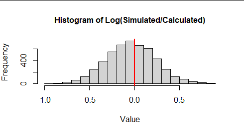
I generated a random $2\times 2$ Complex covariance matrix $\mathbf Q,$ computed $Q(\mathbf z)$ for $100$ iid standard Normal complex vectors $\mathbf z,$ and estimated their variance. Upon repeating this five thousand times I obtained an empirical representation of this distribution. If the preceding result is correct, then the ratio of each of these variance estimates to the calculated variance should be centered at zero. Here is the histogram

It's exactly as expected. I repeated this process several times for $2\times 2$ through $5\times 5$ Complex covariance matrices and observed comparable results.
To illustrate the block matrix notation used above, here are the computer representations of $\mathbf Q$
              [,1]          [,2]
[1,]  0.203+0.000i -0.211+0.204i
[2,] -0.211-0.204i  0.600+0.000i
and $\mathbf Q_{\Re}$
       [,1]   [,2]   [,3]   [,4]
[1,]  0.203 -0.211  0.000 -0.204
[2,] -0.211  0.600  0.204  0.000
[3,]  0.000  0.204  0.203 -0.211
[4,] -0.204  0.000 -0.211  0.600
for the original simulation. Comparing them will make their relationship clear.
Here is the R code used for this check.
#
# Create real symmetric and antisymmetric matrices.
#
set.seed(17)                          # Comment out to produce different random results
n <- 2                                # The complex dimension, 1 or greater
A <- cov(matrix(rnorm(2*n^2), ncol=n))
B <- matrix(rnorm(n^2, 0), n); B <- B - t(B)
while(TRUE) {
  #
  # Verify they represent a Complex covariance.
  #
  Q.Re <- rbind(cbind(A, -B), cbind(B, A))
  if(min(eigen(Q.Re, only.values = TRUE)$values) >= 0) break
  B <- B / 2 # Shrink B and try again
}
#
# Represent it as a Complex hermitian matrix.
#
Q <- A + B * 1i
#
# Verify it is hermitian.
#
if(1 + sum(Mod(Q - Conj(t(Q)))) != 1) stop("Q is not hermitian.")
#
# Compute the variance.  (This is the main result.)
#
var.Q <- 4 * (sum(diag(A %*% A)) - sum(diag(B %*% B)))
#
# Generate standard Complex normal vectors.
#
N.sim <- 1e2
X <- replicate(5e3, {
  XY <- matrix(rnorm(2*n * N.sim), N.sim)
  Z <- XY[, seq_len(n), drop=FALSE] + XY[, seq_len(n) + n, drop=FALSE] * 1i
  #
  # Compute the form for each vector.
  # Because Q is hermitian, the result will be real, so we store it that way.
  #
  q <- Re(apply(Z, 1, function(z) Conj(z) %*% Q %*% z))
  #
  # Report its variance.
  #
  var(q)
})
hist(log(X / var.Q), xlab="Value",
     main="Histogram of Log(Simulated/Calculated)", cex.main=1)
abline(v = 0, col="Red", lwd=2)
#
# Display the matrices of the form.
#
print(round(Q, 3))    # The n X n complex matrix
print(round(Q.Re, 3)) # The equivalent 2n X 2n real matrix

