The moose must flow, but how?

Question

Background

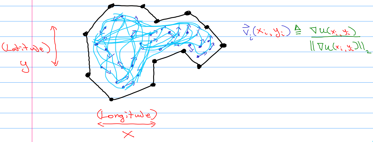
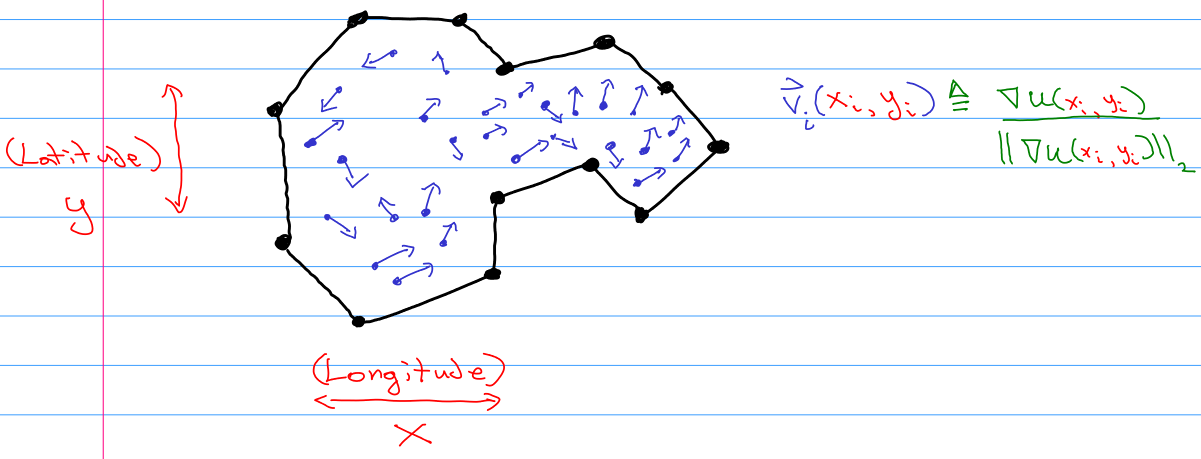
Suppose I collected a data set of the latitude and longitude of moose tracks within an irregular polygon, and also took a compass bearing of the direction that the hooves pointed in.

Image Credit: © Galen Seilis 2022 (used with permission)

Also suppose that the spatial sampling intensity is approximately uniform. The study area is small enough to safely ignore the curvature of the Earth, if desired.

This gets us very close to having a vector field over $\mathbb{R}^2$, only that there is not a clear notion of magnitude. To account for this I define each observation $\vec{v}_i$ to be the normalized gradient at that point in space of some hypothetical field $u : \mathbb{R}^2 \mapsto \mathbb{R}$.

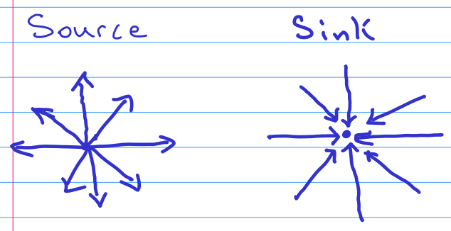
I would like to take on the assumption that there exist no sources or sinks in the gradient of the field $u$. This is due to the fact that moose come and go from the potential study area. While of course moose are born and die somewhere, I want to assume that these events are rare enough to be ignored in my model. Visually this means that neither of the following two patterns occur at any point:

Because of how I defined the observations to be the normalized gradient, I was willing to assume that the gradient isn't the zero vector anywhere anyways. This precludes other field patterns as well.

---

Other Considerations

• At the moment I do not have a well-posed problem.
• The goal is to produce plausible patterns of flow of moose through a small area.
• Sometimes moose tracks are plausibly from the same individual due to being aligned and close together, but usually the tracks are relatively isolated.
• There are plenty of machine learning approaches that I could use to estimate a map $\mathbb{R}^2 \mapsto \mathbb{R}^2$, but I would rather use differential equations for understandability.
• At a boundary point the gradient of $u$ could be perpendicular, parallel, or neither to boundary itself.
• I am not modeling time dependence because estimating the age of a track is quite difficult.
• I have started with assuming it is a function rather than a multivalued function, but a random vector is a reasonable way to go. The former might work if in practice even partially overlapping tracks are not exactly on top of each other. But the latter makes sense in that a given moose might go different directions from the same point depending on unmodeled details of its environment, or that distinct moose could have different brains or perceptions and consequently decide to walk different ways from the same point. Frank's point about crossing paths is excellent: namely that the likely existence of crossing paths precludes the existence of a single-valued vector field.
• I have not decided what is reasonable to assume about the curl; I will think more on it. As Frank pointed out, the curl of the gradient of a field must be zero.
• Random walks on $\mathbb{R}^2$ might be fruitful. The more explainable the better, but I don't mind sprinkling in a little bit of noise from a stochastic process.
• The ultimate goal is to estimate likely paths that the moose are taking into and then out of the bounded region.
• Whuber raises a good point that specific paths are followed by the moose. In theory there should be no vectors where the moose did not go. The difficulty is we do not know where the moose have gone, and wish to infer it.
• SextusEmpiricus suggested that a flux formulation is promising for resolving the problem of crossing paths.
• My guess is that there are probably zero moose in the bounded region on a given day. What I suspect happens is that moose occasionally pass through the area as they browse.
• Sometimes it is possible to tell if tracks are 'extremely' fresh, but in general track ages are not reliably guessed (by me anyway).

---

Question

What model (and boundary conditions if applicable) would be suitable for modeling the flow of moose through a bounded region?

Answer 1

As you have already pointed out, the question is whether you are dealing with a vector field $v$ from your polygon $P$ to $\mathbb{R}^2$, $v:P \to \mathbb R^2$, and since it is supposed to be normalized, your field maps to the unit circle $\mathbf{S}^1$, i.e. $v:P\to\mathbf{S^1}$.

First, let's consider the idea of a gradient field: Note that every vector field that is a gradient field must have zero $curl$, $curl(v) = 0$. And since moose are probably expected to, at least sometimes, walk loops, a gradient field might not be an appropriate model.

Also, moose tracks will probably cross, which means that you don't even have a proper map from your polygon $P$ to $\mathbf S$, so you don't even have a proper vector field.

So then: what could be a proper model? The first step would be to answer the question of what you actually want to achieve, what is your ultimate goal? Do you want to predict where a moose will be in the future? Do you want to have a (time-dependent) "moose density function"? Do you want to classify moose tracks?

Answer 2

Windy moose

You may have few data points to really "model" this. But this does not mean that you could not see the patterns in data.

The trick is that, instead of a spherical cow, you may generalize your beloved moose as wind, and each footprint as a weather station that indicates the observed direction on each point.

With such simplifications in place, you could generate a streamline or quiver plot to see the flow and extract the model.

Answer 3

My thoughts from an ecologist's perspective, especially in the context of:

The ultimate goal is to estimate likely paths that the moose are taking into and then out of the bounded region.

Movement ecology

I mentioned this in a comment, but movement ecology might be the place to look. It focuses a lot on movement data, particularly from GPS trackers, but it's also a very young field. I'm not sure if the theoretical foundation is there yet to go from something like GPS data (which has temporal information, possibly speed acceleration info as well) to what you have (no temporal information, so you don't know the order of your tracks). Unfortunately, I only have a superficial familiarity with it, so I can't point to specific types of modeling/statistical analyses. But just a comment, you might be able to infer speed (or the magnitude of the vectors) by the stride length if you have enough tracks together in a sequence.

Landscape ecology

Depending on your goals and other types of data you might have access to, you could look at landscape ecology for inspiration. A very common goal of ecologists is to understand connectivity in landscapes, usually focused on a particular species, which is important for conservation planning. Connectivity in the landscape is directly related to movement. Low connectivity = low movement potential.

Enter Circuit Theory (the ecological version, which is based on electrical circuit theory). In principle, if you have environmental data relevant to your species, you can create a resistance (or conductance) map specific for your species. For example, things like water and tree cover might indicate low resistance areas for moose, since that's what they generally need to survive, whereas a boulder field might be high resistance (they are more likely to go around it rather than through it). With that single resistance map, you can then model flow and connectivity to predict where your organism might move. Typically, this is based on a random-walk model due to its simplicity.

With environmental data, your moose tracks can potentially be used to create a species distribution model. This in turn can be used as a conductance map for circuit theory. The idea being that if an area is considered "good" for the species, then it's probably easier for them to move through it as well. The problem is that species distribution modeling is a huge and complex topic.

The most well known tool in (ecological) circuit theory might be Circuitscape. There are a ton of research papers and reports that utilize it. More recently, someone I know developed a generalization of circuit theory that incorporates absorption (e.g., mortality), and I developed the samc R package for it. Specifically, it allows you to calculate things like the probability of reaching a particular point, how many times an individual is expected to visit a point, how long it's expected to take to reach a point, how long an individual is expected to survive, etc.

There is overlap between movement and landscape ecology, including incorporating the movement data with correlated random-walks, which can then be incorporated into circuit theory (something I hope to incorporate as an option in my package in the future).

Answer 4

Not an answer, just an extended comment.

First, if you have no temporal data and it can be assumed that not all tracks were found, some could have been damaged, etc, then it is not possible to exactly recreate the path. Only the approximate, "educated guesses" are possible.

If you look at the picture you posted, there are several possibilities for solving it.

• You have a collection of points visited by the moose. You probably can make an assumption that if two tracks heading in a similar direction are close to each other, they are more likely to follow one after another. If you frame it like this, it is a variation of traveling salesman problem, isn't it?

• Travelling salesman would find a single path. Given the noisy nature of the data, this might not be the best solution. Another approach might be to simulate possible paths (the direction of the vector tells you how they should start and end) between all the pairs of points, where the importance of each path, or probability of sampling it, would be inversely proportional to the length of the path. In such a case, you would find regions with many overlapping paths or higher importance weight of all the paths within this area, to find the most likely ones. Here "likely" path would be such that resulted from overlapping many simulated paths.

  This might be more challenging technically (how would you generate the curves? how would you judge if they are plausible?), but to prove yourself that the approach might make sense try drawing the lines by hand first. As you can see from the image below, after drawing a bunch of "random" lines patterns start to emerge. Drawing them by hand is not the best idea, because people are very bad at generating "random" things, we seek and force patterns, so you would fast start generating "random" paths that fit your hypothesis. This is just an example to show how sampling random paths could be useful here.

Answer 5

Building on the answer of Betterthan Kwora, here is one possible approach.

You can view your vector field as a function $\{(x_i, y_i)\}_{1 \le i \le n} \subset \mathbb{R}^2 \rightarrow [0, 2\pi]$, because each moose vector has unit length. You can use interpolation to extend this to a function defined on the whole of $\mathbb{R}^2$, for example by using radial basis functions. Once you have this extended vector field, you can simulate possible paths.

Here is an implementation of the idea in R. First, here is a function to simulate some data. By default, these moose tend to move from east to west:

simulate_moose <- function(N, x1=1, y1=1, a1=2, a2=2){
  # simulate some data in the rectangle [0, x1] x [0, y1]
  # N: number of data points
  # a1, a2: parameters of beta distribution (bias moose direction)
  # default "ground truth" is that moose are moving westwards in this example
  
  # choose start point for each vector
  x <- runif(N) * x1
  y <- runif(N) * y1
  
  # choose a direction for each vector
  angles <- rbeta(N, a1, a2) * 2 * pi
  vx <- cos(angles)
  vy <- sin(angles)
  
  list(x=x, y=y, vx=vx, vy=vy)
}

Here is a function to fit a vector field to moose data:

fit_vector_field <- function(moose_data, r=0.2){
  
  # fit vector field using normals
  # larger r = more smoothing
  
  x0 <- moose_data$x
  y0 <- moose_data$y
  vx0 <- moose_data$vx
  vy0 <- moose_data$vy
  
  # get angle from vx and vy values in data
  theta <- acos(vx0)
  theta[vy0 > 0] <- -theta[vy0 > 0]
  
  # convert angles to real number in range (-inf, inf)
  z <- tan((theta - pi)/2)
  
  fitted_field <- function(x, y){
    # get weights using Gaussian - invariant to rotations
    w <- (2 * pi * r^2)^-0.5 * exp(( -(x - x0)^2 -(y - y0)^2)/(2 * r^2))
    w <- w/sum(w)
    
    # use weights to estimate tan of desired angle at desired point (x, y)
    z_est <- sum(w * z)
    
    # convert back to an angle
    theta_est <- 2 * atan(z_est) + pi
    
    # convert from angle to (vx, vy) direction vector
    list(vx=cos(theta_est), vy=sin(theta_est))
  }
  
  fitted_field  
}

Here is a plotting function and an example:

plot_vector_field <- function(vector_field, vlength=1, ...){
  
  # plot the moose data using a circular head for the vectors
  x <- vector_field$x
  y <- vector_field$y
  vx <- vector_field$vx * vlength
  vy <- vector_field$vy * vlength
  
  do.call(plot, c(list(x=x, y=y, xlab="", ylab="", cex=0), list(...)))
  for (i in 1:length(x)){
    segments(x[i], y[i], x[i] + vx[i], y[i] + vy[i])
    points(x[i] + vx[i], y[i] + vy[i], pch=19)
  }
}

simulate_moose_path <- function(fitted_field, start_x, start_y, N_steps, stepsize){
  
  # simulate a path from start point (start_x, start_y)
  # use N steps of size stepsize
  
  x <- y <- rep(0, N_steps)
  
  x[1] <- start_x
  y[1] <- start_y
  
  for (i in 2:N_steps){
    
    pred <- fitted_field(x[i-1], y[i-1])
    x[i] <- x[i-1] + pred$vx * stepsize
    y[i] <- y[i-1] + pred$vy * stepsize
  }
  list(x=x, y=y)
}

# example
set.seed(42)
moose_data <- simulate_moose(60)
fitted_field <- fit_vector_field(moose_data)
plot_vector_field(moose_data, vlength=0.1, xlim=c(-0.1, 1.1), ylim=c(-0.1, 1.1))
for (i in -1:5){
  for (j in -1:5){
    path <- simulate_moose_path(fitted_field, i/5, j/5, 50, 0.1)
    lines(path, col="blue", lwd=2)
  }
}

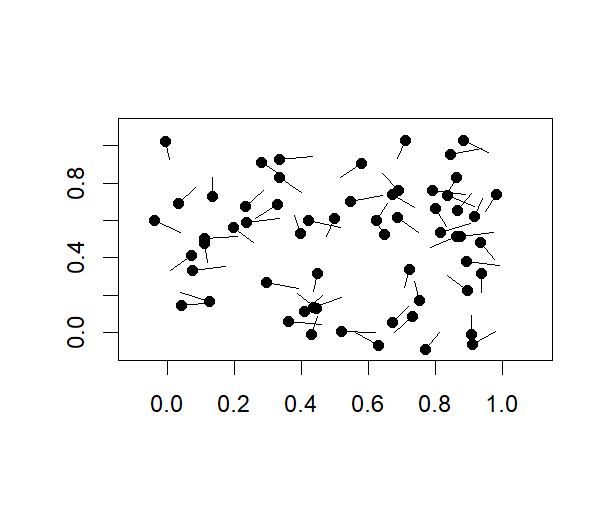
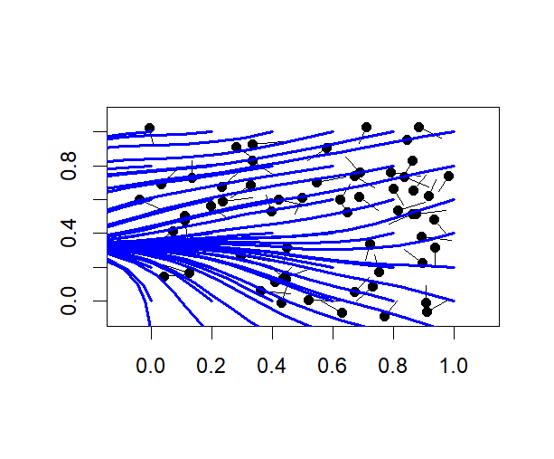
The simulated data: and the simulated paths: Perhaps this naive approach might be useful if you want to get a quick check of the paths you get from more sophisticated/rigorous methods.

Answer 6

This approach of finding best-fit vector paths through a bounded volume with directed point measurements is the overall principle of Diffusion Tensor Imaging. There is a large volume of methodology and mathematics around finding paths under these constraints. An example of an introduction article: https://www.ncbi.nlm.nih.gov/pmc/articles/PMC3163395/ explains the general principle of anisotropic measurements in voxels (or pixels, in your case).

More advanced approaches can account for crossing fibers, which is more likely in your case since you only have two dimensions. These methods are generally validated against real-world physical brains, so you can have some confidence that they have validity within their constraints.

I hope you can adapt these principles to your moose-tracking problem.

Answer 7

Let's first propose a fairly general description of the underlying moose motion, and then consider how the hoofprint observations can help infer the specific dynamics.

We start with an assumption that the observations cover either a large enough number of moose, or a long enough period of time, so that a continuous moose distribution is applicable. We can then apply concepts from statistical mechanics such as the Boltzmann equation -- granted that we don't know a priori what drives the motion of moose, so we can't fill in the equivalent of "forces acting on molecules", but we can describe the counting and kinematics given merely that each moose has a position and velocity and follows a continuous path in space.

At any given time, the expected number of moose located in a small box $\Delta x\, \Delta y$ around $(x, y)$ and with velocity in a small box $\Delta\xi\, \Delta\eta$ around $(\xi, \eta)$ equals $$\Delta x\, \Delta y\, \Delta\xi\, \Delta\eta\, f(x, y, \xi, \eta),$$ which defines the distribution function $f$. A consequence is that the expected number of moose located in $\Delta x\, \Delta y$ with any velocity equals $$\Delta x\, \Delta y \int_{\mathbb{R}^2} d\xi\, d\eta\, f(x, y, \xi, \eta) \equiv \Delta x\, \Delta y\, \rho(x, y).$$ We call $\rho$ the density of moose.

By the definition of velocity, each moose satisfies $dx/dt = \xi$, $dy/dt = \eta$. In a short time interval $\Delta t$, the expected net number of moose that cross (from left to right, minus from right to left) a "vertical" line segment $\Delta y$ around $(x, y)$ is the expected number of moose with any velocity $(\xi, \eta)$ and located in a box $(\xi\, \Delta t)\, \Delta y$, since this box of moose moves horizontally by $\xi\, \Delta t$ and crosses the line segment. Thus, this expected number of crossings equals $$\Delta t\, \Delta y \int_{\mathbb{R}^2} d\xi\, d\eta\, \xi\, f(x, y, \xi, \eta) \equiv \Delta t\, \Delta y\, \alpha(x, y).$$ Likewise, the expected net number of moose that cross (from bottom to top, minus from top to bottom) a "horizontal" line segment $\Delta x$ around $(x, y)$ equals $$\Delta t\, \Delta x \int_{\mathbb{R}^2} d\xi\, d\eta\, \eta\, f(x, y, \xi, \eta) \equiv \Delta t\, \Delta x\, \beta(x, y).$$ We call $(\alpha, \beta)$ the flux of moose. It is a useful vector field that we would like to infer, because it quantifies the net motion of moose in any direction: The crossings of an oblique line segment are given by an appropriate linear combination of $\alpha$ and $\beta$.

Now, let's assume both that the moose distribution function is steady over time and that moose are neither created nor destroyed. Then, by setting to zero the expected net number of moose that cross (out of minus into) the four sides of a box $\Delta x\, \Delta y$ around $(x, y)$, we obtain $$\Delta t\, \Delta y\, \bigl(\alpha(x + \tfrac{1}{2}\Delta x, y) - \alpha(x - \tfrac{1}{2}\Delta x, y)\bigr) + \Delta t\, \Delta x\, \bigl(\beta(x, y + \tfrac{1}{2}\Delta y) - \beta(x, y - \tfrac{1}{2}\Delta y)\bigr) = 0.$$ Upon dividing by $\Delta t\, \Delta x\, \Delta y$ and taking the limit of a very small box, it follows that $$\frac{\partial\alpha(x, y)}{\partial x} + \frac{\partial\beta(x, y)}{\partial y} = 0.$$ This "continuity equation" says that the flux has zero divergence. This is the rigorous formulation of "no sources or sinks". Note that sources and sinks could exist even for a vector field that is nowhere zero, so ruling out the symmetric source and sink patterns sketched in the question is not sufficient.

Now, what do the hoofprints represent? Each hoofprint tells us that a moose was present at a point $(x, y)$ and had a velocity in a specific direction, $(\xi, \eta) \propto (\cos\theta, \sin\theta)$. Unfortunately, this does not directly allow us to estimate any sort of distribution function, because moose may leave hoofprints at various rates. It would be easier if every moose always took a step every 1 second, say; then we would be uniformly sampling every moose's position and direction. But if moose may tend to pause in a certain area and take more time between steps, then the number of hoofprints will not adequately indicate the increased probability of finding moose there.

It may be possible, though, to combine the hoofprint information with the kinematic properties derived above, and obtain a useful characterization of the moose flux. While moose at the same location can move in different directions (crossing paths), suppose they tend to move mostly in a similar direction. This will result in the flux $(\alpha, \beta)$ also tending to point in that direction. In the limit in which moose at each point $(x, y)$ have a unique velocity $(\xi, \eta)$, the flux is $(\alpha, \beta) = (\rho\xi, \rho\eta)$; upon relaxing this condition, we can still use the typical direction of $(\xi, \eta)$ around $(x, y)$ as an approximation of the direction of $(\alpha, \beta)$.

In addition, although the sampling of hoofprints is nonuniform as noted above, it is still true that areas with no moose ($\rho = 0$) will have no hoofprints as well as zero flux. Thus, it is useful to include the number of nearby hoofprints in scaling an approximation of $(\alpha, \beta)$.

So, we can consider modeling the flux as $$\bigl(\alpha(x, y), \beta(x, y)\bigr) = q(x, y) \sum_i (\cos\theta_i, \sin\theta_i)\, K(x - x_i, y - y_i),$$ i.e., a scalar function $q$ (which accommodates unknown factors such as local moose speed) times a kernel density estimate of the typical local direction. The kernel will tend to generate the noted correlation of flux with local hoofprint density, enabling the function $q$ to be smoother. The choice of kernel shape and width is an empirical matter.

For the one unknown function $q(x, y)$, we require one partial differential equation, which was derived above: $$\frac{\partial\alpha(x, y)}{\partial x} + \frac{\partial\beta(x, y)}{\partial y} = 0.$$ That is, we could try using the continuity equation to solve numerically for the unknown magnitude of the flux at each point. Further investigation would be needed regarding boundary conditions and well-posedness.

This approach is somewhat similar to how the question proposes treating the local direction $(\cos\theta, \sin\theta)$ as the result of normalizing an underlying vector field, but there is no reason that the underlying field needs to be the gradient of a scalar.

Answer 8

It appears that you can break this down into separate problems.

First, you can attempt to infer a moose movement vector for each point in your polygon. This will take the form of learning a function $f: \mathbb{R}^2 \mapsto \mathbb{R}^2$. Better yet, this would be a stochastic function, yielding a distribution over movement vectors for each location.

Second, given your function $f$, you can attempt to infer likely trajectories. To infer trajectories, you'd simply simulate them (with sampling, if your function is stochastic), perhaps with your observations as initial points. There would be complications involving choice of step size, but overall this is not hard.

Third, you'd need to fit differential equations to these trajectories. Given a family of ODEs with a certain parameterization, estimation of parameters is also not so hard, with many possible approaches in the literature.

Answer 9

Moose density

While other answers have taken more sophisticated approaches I'd suggest neglecting the vector data for a moment - does your sampling mean that you can estimate the density of moose (regardless of direction) from your observed tracks? That will in itself be worthwhile.

You can then add data points using the vectors - if you have your set of points X and vectors V, you have an initial density from X itself, but you can enrich this by using X union X + V union X - V. This may work better if elements of V are not normalised, however.

If you have enough data you can also estimate the density of moose travelling in each direction, as a first step towards the wind models mentioned in other answers - this sort of approach isn't fancy but it does handle 'contradictory data' without conflict.

Answer 10

One thing you could consider would be a discrete model. The idea is this: using your measurement points, make a Voronoi diagram to divide your polygon up into cells. The direction measurement gives a directed graph on the cells, as it points to a unique adjacent cell, and you could consider moose to travel deterministically as prescribed by this graph. (Or, if you want to be a little more realistic, you could consider some distribution on directions whose mode is the measured direction, and consider moose to travel stochastically according to the resulting weighted graph.)

One nice thing about this formulation is that it enforces your "no sinks, no sources" property: since each cell has exactly one other cell that it "points" to, your moose will never get stuck with no directions to go (a sink) and will never suffer from choice paralysis (a source). Your poor memoryless moose might get stuck wandering in a cycle forever, though!