No gradient for one parameter on the first iteration of gradient descent

Question

Say we have a dataset $D$ of 2-tuples $(x, y)$ where $y$ is the target variable and a function $f_\theta$:

$$ D = \{(1, 3), (2, 5), (3, 8), (4, 6), (5, 9)\},\quad f_\theta(x) = \theta_0 + \theta_1 x. $$

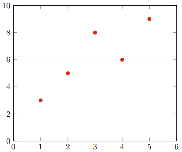
Arbitrarily, I chose $\theta_0$ (the $y$-intercept) to be the mean of the target variable, which is $6.2$, and $\theta_1$ (the slope of the line) to be $0$, such that the representation of the function is a line as seen below (data points are in red):

I wanted to perform linear regression using gradient descent and mean squared error (MSE). The MSE is

$$ MSE(D, f_\theta) = \frac{1}{2M} \sum_{i = 1}^{M} (f_\theta(x_i) - y_i)^2 $$

and so, for this dataset, the gradient on the first iteration is

$$ \nabla_\theta MSE(D, f_\theta) = - \frac{1}{5} \sum_{i = 1}^{5} x_i(y_i - \theta^\top x_i) = \begin{bmatrix}0.0\\-2.6\end{bmatrix} $$

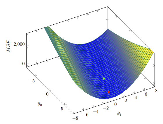
I found it weird that the first parameter $\theta_0$ had no gradient, so first of all I calculated (using the closed form) the optimal parameters for MSE, which yielded $\theta^\ast = \begin{bmatrix}2.3 & 1.3\end{bmatrix}^\top$. I also calculated the MSE function for the dataset and plotted it:

$$ MSE(D, f_\theta) = \frac{1}{2 \cdot 5} \sum_{i = 1}^{5} (f_\theta(x_i) - y_i)^2 = \frac{1}{10}(5x^2 + x(30y - 62) + 55y^2 - 212y + 215) $$

The red point corresponds to the starting parameters, $\theta = \begin{bmatrix}6.2 & 0\end{bmatrix}^\top$, and the green point corresponds to the optimal parameters, $\theta^\ast = \begin{bmatrix}2.3 & 1.3\end{bmatrix}^\top$. Note that only in the first iteration of gradient descent was the gradient for $\theta_0 = 0$; in the following epochs $\theta_0$ started to converge towards $2.3$.

Question: from the plot above, it is clear that $\theta_0$ "has to move" so that the red dot (the starting parameters) can approximate the green dot (the global optimum). Since the MSE is convex, how come the first iteration of gradient descent as calculated above yields no gradient for $\theta_0$?

---

I guess I can see from the first plot why the gradient for $\theta_0$ would be 0: since I initialized $\theta_0 = 6.2$, it already minimizes the squared errors for that variable (for $\theta_1 = 0$). My confusion stems from the plotted MSE. I usually picture the parameters as "rolling downhill" towards the minimum in a convex function, and I can't seem to wrap my head around why we wouldn't also "roll" along the $\theta_0$ axis in that first iteration.

---

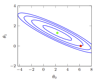
After reading the accepted answer, I thought I'd add a countour plot of the loss:

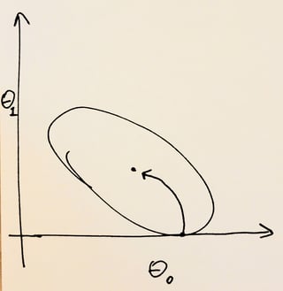
Since the gradient is orthogonal to the level curve, it is easy to see how we would move only along $\theta_1$ when starting from the red dot.

Answer 1

Yes, you do roll downhill from the initial point to the optimum, but this doesn't happen in a straight line.

It might be easier to see what's going on if we plot a level contour of the loss, all points on the ellipse below result in the same MSE. (level curves of a convex quadratic are elliptical)

We start at the very bottom of the ellipse where $\theta_1 = 0$, and head toward the optimum at the center of the ellipse. But the gradient is always perpendicular to the level curve, which means where $\theta_1 = 0$ is tangent to the ellipse, the gradient points straight up.