19
$\begingroup$

Are the phi and Matthews correlation coefficients the same concept? How are they related or equivalent to Pearson correlation coefficient for two binary variables? I assume the binary values are 0 and 1.


The Pearson's correlation between two Bernoulli random variables $x$ and $y$ is:

$$ \rho = \frac{\mathbb{E} [(x - \mathbb{E}[x])(y - \mathbb{E}[y])]} {\sqrt{\text{Var}[x] \, \text{Var}[y]}} = \frac{\mathbb{E} [xy] - \mathbb{E}[x] \, \mathbb{E}[y]}{\sqrt{\text{Var}[x] \, \text{Var}[y]}} = \frac{n_{1 1} n - n_{1\bullet} n_{\bullet 1}}{\sqrt{n_{0\bullet}n_{1\bullet} n_{\bullet 0}n_{\bullet 1}}} $$

where

$$ \mathbb{E}[x] = \frac{n_{1\bullet}}{n} \quad \text{Var}[x] = \frac{n_{0\bullet}n_{1\bullet}}{n^2} \quad \mathbb{E}[y] = \frac{n_{\bullet 1}}{n} \quad \text{Var}[y] = \frac{n_{\bullet 0}n_{\bullet 1}}{n^2} \quad \mathbb{E}[xy] = \frac{n_{11}}{n} $$


Phi coefficient from Wikipedia:

In statistics, the phi coefficient (also referred to as the "mean square contingency coefficient" and denoted by $\phi$ or $r_\phi$) is a measure of association for two binary variables introduced by Karl Pearson. This measure is similar to the Pearson correlation coefficient in its interpretation. In fact, a Pearson correlation coefficient estimated for two binary variables will return the phi coefficient...

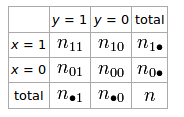
If we have a 2 × 2 table for two random variables $x$ and $y$

enter image description here

The phi coefficient that describes the association of $x$ and $y$ is $$ \phi = \frac{n_{11}n_{00} - n_{10}n_{01}}{\sqrt{n_{1\bullet}n_{0\bullet}n_{\bullet0}n_{\bullet1}}} $$

Matthews correlation coefficient from Wikipedia:

The Matthews correlation coefficient (MCC) can be calculated directly from the confusion matrix using the formula: $$ \text{MCC} = \frac{ TP \times TN - FP \times FN } {\sqrt{ (TP + FP) (TP + FN) (TN + FP) (TN + FN) } } $$

In this equation, TP is the number of true positives, TN the number of true negatives, FP the number of false positives and FN the number of false negatives. If any of the four sums in the denominator is zero, the denominator can be arbitrarily set to one; this results in a Matthews correlation coefficient of zero, which can be shown to be the correct limiting value.

$\endgroup$
0

3 Answers 3

19
$\begingroup$

Yes, they are the same. The Matthews correlation coefficient is just a particular application of the Pearson correlation coefficient to a confusion table.

A contingency table is just a summary of underlying data. You can convert it back from the counts shown in the contingency table to one row per observations.

Consider the example confusion matrix used in the Wikipedia article with 5 true positives, 17 true negatives, 2 false positives and 3 false negatives

> matrix(c(5,3,2,17), nrow=2, byrow=TRUE)
     [,1] [,2]
[1,]    5    3
[2,]    2   17
> 
> # Matthews correlation coefficient directly from the Wikipedia formula
> (5*17-3*2) / sqrt((5+3)*(5+2)*(17+3)*(17+2))
[1] 0.5415534
> 
> 
> # Convert this into a long form binary variable and find the correlation coefficient
> conf.m <- data.frame(
+ X1=rep(c(0,1,0,1), c(5,3,2,17)),
+ X2=rep(c(0,0,1,1), c(5,3,2,17)))
> conf.m # what does that look like?
   X1 X2
1   0  0
2   0  0
3   0  0
4   0  0
5   0  0
6   1  0
7   1  0
8   1  0
9   0  1
10  0  1
11  1  1
12  1  1
13  1  1
14  1  1
15  1  1
16  1  1
17  1  1
18  1  1
19  1  1
20  1  1
21  1  1
22  1  1
23  1  1
24  1  1
25  1  1
26  1  1
27  1  1
> cor(conf.m)
          X1        X2
X1 1.0000000 0.5415534
X2 0.5415534 1.0000000
$\endgroup$
2
  • $\begingroup$ Thanks, Peter! Mathematically, why are phi and Mathew equivalent to Pearson for two binary random variables? $\endgroup$
    – Tim
    Commented May 18, 2013 at 1:36
  • $\begingroup$ If you take the definition of the Pearson correlation and manipulate it so it refers to counts rather than to sums of the differences between individual observations and the means, you get the Matthews formula. I haven't actually done this, but it must be reasonably straightforward. $\endgroup$ Commented May 18, 2013 at 1:44
4
$\begingroup$

Firstly, there was a typo error in the question: $\mathbb{E}[xy]$ is not $\displaystyle \frac{n_{\bullet 1}n_{1\bullet}}{n^2}$ but rather

$$ \frac{n_{11}}{n} \times 1 \times 1 + \frac{n_{10}}{n}\times 1 \times 0 + \frac{n_{01}}{n} \times 0 \times 1 + \frac{n_{00}}{n} \times 0 \times 0 = \frac{n_{11}}{n} $$

Secondly, the key to showing that $\rho = \phi$ is

$$ n_{11} n - n_{1\bullet} n_{\bullet 1} = n_{11} (n_{01} + n_{10} + n_{11} + n_{00}) - (n_{11} + n_{10}) (n_{11} + n_{01}) \\ = n_{11} n_{00} - n_{10} n_{01} $$

$\endgroup$
1
$\begingroup$

I want to note that the phi coefficient $\phi$ (MCC is just a synonym for it) will be equal to the Pearson correlation coefficient $r$ not only when random variables $X$ and $Y$ take values from the set $R = \{0,1\}$ but also in the following cases:

  1. When $X$ and $Y$ take values from any other numeric binary set, for example, from $R = \{-1,1\}$ or $R = \{5.5,3.7\}$, etc.

  2. When random variable $X$ takes values from the set $R_X = \{x_1, x_2\}$ and random variable $Y$ takes values from the set $R_Y = \{y_1, y_2\}$ (this case may correspond to a situation when $X$ and $Y$ are two nominal variables with two categories each, and we mapped the categories into some different numeric values; such mapping is, of course, not unique) if the contingency table is built in such a way that numbers $\mathrm{max}(x_1,x_2)$ and $\mathrm{max}(y_1,y_2)$ are the names of the 1st row and 1st column of the table respectively (or the names of the 2nd row and the 2nd column of the table respectively).


The proof is given below.

A key mathematical property of the Pearson correlation coefficient is that it is invariant under separate changes in location and scale in the two variables. That is, we may transform $X$ to $a + b X$ and transform $Y$ to $c + d Y$, where $a, b, c, d$ are constants with $b, d \gt 0$, without changing the correlation coefficient (this holds for both the population and sample Pearson correlation coefficients). So if we have $R_X = \{x_1,x_2\}$ and $R_Y = \{y_1,y_2\}$ there always exist linear mappings $$f: X \to U = \frac{-x_1 + X}{x_2 - x_1}, \quad g:Y \to V = \frac{-y_1+Y}{y_2-y_1},$$ they map $R_X \overset{f}{\to} \{0,1\}, \, R_Y \overset{g}{\to} \{0,1\}$.

Using them, we get that Pearson's $r(\mathbf{x},\mathbf{y}) = r(f(\mathbf{x}), \, g(\mathbf{y})) = r(\mathbf{u}, \mathbf{v})$, where $\mathbf{u}, \mathbf{v} \in \{0,1\}^n$. Next, user ryan_tt proved in his post that $r(\mathbf{u}, \mathbf{v}) = \phi(\mathbf{u}, \mathbf{v})$. Hence, $$r(\mathbf{x},\mathbf{y}) = \phi\left(\frac{-x_1 + \mathbf{x}}{x_2 - x_1}, \frac{-y_1+\mathbf{y}}{y_2-y_1} \right), \qquad \forall \mathbf{x},\mathbf{y} \in \mathbb{R}^n.$$

$\endgroup$

Your Answer

By clicking “Post Your Answer”, you agree to our terms of service and acknowledge you have read our privacy policy.

Not the answer you're looking for? Browse other questions tagged or ask your own question.