3
$\begingroup$

I'm looking to test explanatory variables that might have quadratic rather than linear relation to the dependent variable. I have read in several places that this could be done using the squared (^2) values of the explanatory variables. However, in all the examples I found online, as well as for my analysis, results for both linear and quadratic regressions were significant (though sometimes opposite -/+).

I can see how both could be correct sometimes but just in case I ran it on a dataset that is obviously linear:

Var1 <- seq(1:51) 
Var2 <- seq(0, 1, 0.02)
Var3 <- Var2^2
Test <- data.frame(cbind(Var1, Var2, Var3))
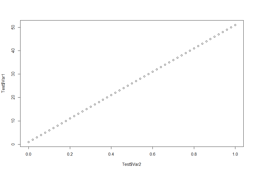
plot(Test$Var2, Test$Var1)

enter image description here

summary(lm(Var1 ~ Var2 + Var3, Test))

Call:
lm(formula = Var1 ~ Var2 + Var3, data = Test)

Residuals:
       Min         1Q     Median         3Q        Max 
-3.801e-14 -1.868e-15  2.200e-17  3.997e-15  1.222e-14 

Coefficients:
              Estimate Std. Error    t value Pr(>|t|)    
(Intercept)  1.000e+00  3.099e-15  3.227e+14   <2e-16 ***
Var2         5.000e+01  1.433e-14  3.489e+15   <2e-16 ***
Var3        -3.977e-14  1.386e-14 -2.869e+00   0.0061 ** 
---
Signif. codes:  0 ‘***’ 0.001 ‘**’ 0.01 ‘*’ 0.05 ‘.’ 0.1 ‘ ’ 1

Residual standard error: 7.668e-15 on 48 degrees of freedom
Multiple R-squared:      1, Adjusted R-squared:      1 
F-statistic: 9.395e+31 on 2 and 48 DF,  p-value: < 2.2e-16

Can anyone explain how is this possible and how should I approach it? What are the circumstances where it should and shouldn't be used?

**Edit: When i run the regression with only the quadratic variable such as

summary(lm(Var1~Var3, data = Test))

I get this result

Call:
lm(formula = Var1 ~ Var3, data = Test)

Residuals:
   Min     1Q Median     3Q    Max 
-9.257 -2.645  1.077  3.317  4.107 

Coefficients:
            Estimate Std. Error t value Pr(>|t|)    
(Intercept)  10.2569     0.7979   12.86   <2e-16 ***
Var3         46.7616     1.7580   26.60   <2e-16 ***
---
Signif. codes:  0 ‘***’ 0.001 ‘**’ 0.01 ‘*’ 0.05 ‘.’ 0.1 ‘ ’ 1

Residual standard error: 3.822 on 49 degrees of freedom
Multiple R-squared:  0.9352,    Adjusted R-squared:  0.9339 
F-statistic: 707.5 on 1 and 49 DF,  p-value: < 2.2e-16

Can anyone explain the logic of the regression I think I'm missing?

$\endgroup$
3
  • 3
    $\begingroup$ The result may say the quadratic factor is statistically significant, but with a value is $10^{-14}$ it is physically insignificant. Probably a result of a floating point rounding error $\endgroup$
    – Dave2e
    Commented Dec 8, 2022 at 2:05
  • $\begingroup$ That's a very good point, thank you, but please see my edit to the question regarding a regression with only a quadratic variable. $\endgroup$ Commented Dec 8, 2022 at 3:02
  • $\begingroup$ I don't think this is a particularly instructive simulated data. Add a bit of noise and you'll get quite different results. $\endgroup$
    – dipetkov
    Commented Dec 10, 2022 at 15:57

2 Answers 2

3
$\begingroup$

The result may say the quadratic factor is statistically significant, but with a value is $10^{−14}$ it is physically insignificant.

I am thinking your question is "Why is there a quadratic coefficient so small and not equal to 0 from the original definition?" To answer this look at your plot. The x range (from 0 to 1) is small and in that range the function is linear. (no curvature). The contribution quadratic (or higher orders) is very small in the range of -1 < x < 1. Since the square of small number is even smaller. ) $.1^2 = 0.01$, thus no contribution.
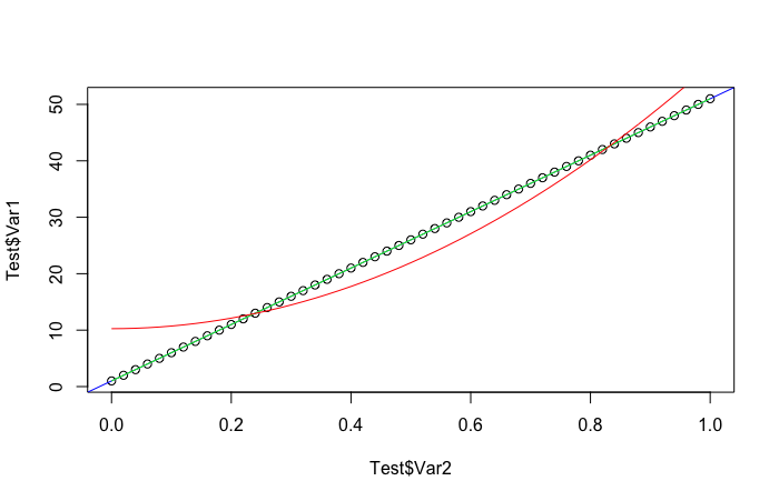
See the blue and green lines below. Both lines are nearly equal.

enter image description here

Now for your second model, fitting a quadratic without the linear term.
The least squares method is finding the best 2 coefficients to minimize the error and the result is the red curve. Again there are 50 data points in a small x-range where the quadratic effect is insignificant and thus still a pretty good linear fit.
In fact you just fit the intercept (without any independent variable) you will still end up with a decent fit.

Hopefully this help cleared up your confusion.

Var1 <- seq(1:51) 
Var2 <- seq(0, 1, 0.02)
Var3 <- Var2^2
Test <- data.frame(cbind(Var1, Var2, Var3))
plot(Test$Var2, Test$Var1)

linear <- lm(Var1 ~ Var2, Test)
summary(linear)
abline(linear, col="blue")

quad <- lm(Var1 ~ Var2 + Var3, Test)
summary(quad)
lines(x=Test$Var2, y=predict(quad, Test), col="green")

quad_lite <- lm(Var1 ~ Var3, Test)
summary(quad_lite)
lines(x=Test$Var2, y=predict(quad_lite, Test), col="red")

intercept <- lm(Var1 ~ 1, Test)
summary(intercept)
$\endgroup$
2
$\begingroup$

Actually, your question is about model selection and not about statistical significance of regression parameters. Although the latter can be, and often is used for reducing a model, it is somewhat dubious for picking the degree of a polynomial, because the variables $x$ and $x^2$ are far from independent and, depending on their range, can be highly correlated:

> x <- -5:5
> cor(x, x^2)
[1] 0
> x <- 0:10
> cor(x, x^2)
[1] 0.9631427

Generally, using higher degree polynomials for fitting will always increase the fitting accuracy (measured by $R^2$ in linear regression) on the data used for fitting, but at some point, it will result in overfitting (i.e.: it will perform poorly on unseen data). To find this turnaround point, different indices can be used, e.g.:

  • the leave-one-out mean squared error or, equivalently, the leave-one-out $R^2$
  • the Akaike Information Criterion (AIC)

For linear models, both criteria are asymptotically equivalent. It is thus easiest to use AIC (which is a builtin R function) to find an appropriate degree: lower AIC is better. Code outline:

for (degree in 1:3) {
    cat(sprintf("degree=%i: AIC=%f\n", degree, AIC(lm(y ~ poly(x,degree), data))))
}
$\endgroup$
2
  • $\begingroup$ The Ramsey RESET test might be usueful to OP. $\endgroup$
    – Roland
    Commented Dec 9, 2022 at 7:07
  • $\begingroup$ Thanks for pointing to this method, of which I have never heard before. Do you know how it compares to AIC based model selection? That this test is not (or rarely?) mentioned in text boooks on linear regression does not necessarily speak against it. It seems, however, to be solely based on in-sample estimates, so I wonder whether Ramsey's test can detect overfitting. Can you elaborate in the ideas in an answer? $\endgroup$
    – cdalitz
    Commented Dec 9, 2022 at 13:18

Your Answer

By clicking “Post Your Answer”, you agree to our terms of service and acknowledge you have read our privacy policy.

Not the answer you're looking for? Browse other questions tagged or ask your own question.