Should adjusted models produce narrower CIs than crude ones? What does it depend on?

Question

I am working on a research project for my Masters in Public Health which compares suicide rates across different time periods. I have done all my analysis in R and from what I can tell everything is fine, but my supervisor has suggested that my adjusted model outputting narrower CI's than my crude model is somehow suspicious. I don't think I have a deep enough understanding of CI's to engage him directly, but I'm pretty sure I've seen other studies where the results look this way.

Is this something I should be worried about? What would determine whether adjusting for confounders would narrow or widen CI's for estimates?

For reference: the models are fitted as below.

crude_model = glm.nb(n ~ year+offset(log(population)), control = glm.control(maxit = 100), data = data2)

adjusted_model = glm.nb(n ~ year+Age_Group+Sex+Day_of_Week+offset(log(population)), control = glm.control(maxit = 100), data = data2)

Answer 1

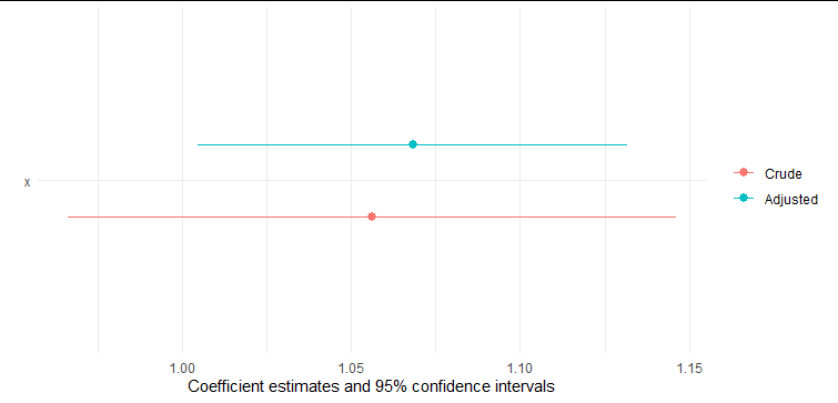
One of the most important reasons to add covariates into a regression model is to explain residual variation in the outcome, and so increase precision in parameter estimates from the model.

So if the covariates "Age Group" and "Day of Week" help to explain residual variance in the outcome measure then your confidence intervals could be smaller than in the crude model.

Consider for example a paired vs an unpaired test. We know that we should expect more precise results (smaller confidence intervals) when we can explain variance using pairing, and you can think of this as if the pairing factor is a covariate being added to a regression model.

Here's a quick simulation of a parameter estimate (for the effect of x on y) becoming more precise when a covariate (z) is added to a model:

 z <- rnorm(1000)
 x <- rnorm(1000)
 y = x + z + rnorm(1000)

 
 m1 = lm(y ~ x)
 m2 = lm(y ~ x+z) 

 modelsummary::modelplot(list("Crude"=m1,"Adjusted"=m2),coef_omit = c(-2)) 

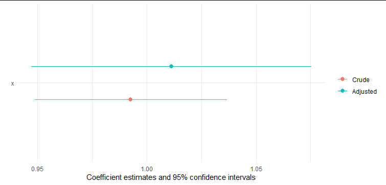
On the other hand, as @whuber points out in the comments, it's possible that adding a covariate will increase the standard errors. Here is a similar situation, but now the covariate z affects the predictor x but has no independent effect on y. If we control for z in our regression estimating the effect of x on y then the precision will be lower:

z <- rnorm(1000)
x <- rnorm(1000) + z
 
y = x + rnorm(1000)
 
m3 = lm(y ~ x)
m4 = lm(y ~ x+z) 
 
modelsummary::modelplot(list("Crude"=m3,"Adjusted"=m4),coef_omit = c(-2)) 

In your case I think the former situation is more likely (although that's down to your understanding of the theory). Adding age group and day of week seems likely to explain variation in suicide rate, but can't really be confounders or explanatory factors for the year variable. So I would guess you'd get more precise estimates of the year effect from the second model.