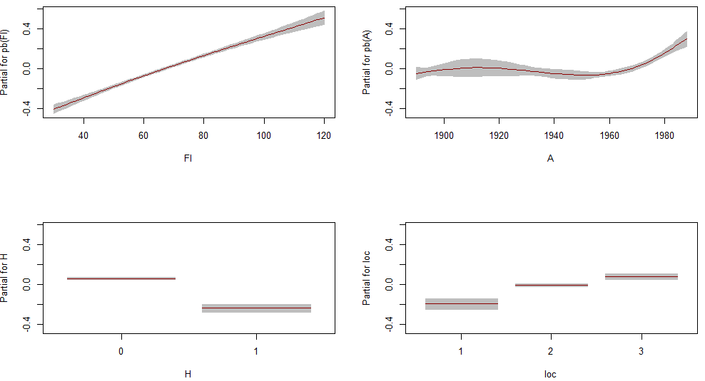
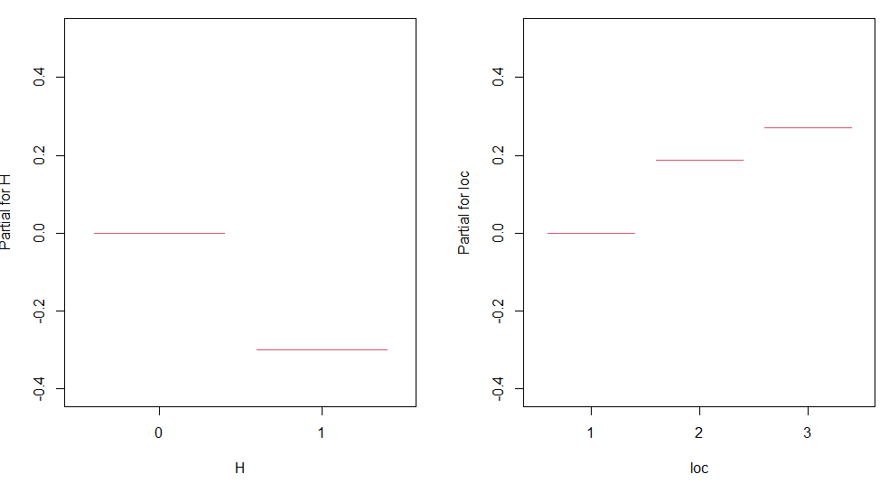
I am interested in plotting the marginal effects in my GAMLSS model. However, what puzzles me a bit is that when using the term.plot() function from the gamlss package I do get estimates for the baseline category of a factor as well. However, when fitting a GAM model with the package mgcv the baseline category is always set to zero, which is also more intuitive to me.
Underneath you can find a worked out example using the rent dataset from the gamlss package. The two factor variables are loc (1 = location below average, 2 = average location, 3 = location above average) and H (0 = no central heating, 1 = central heating) and A (year of construction) as well as Fl (floor space in meters) are modelled as P-Splines.
library(mgcv)
library(gamlss)

r <- gamlss(R ~ pb(Fl) + pb(A) + H + loc, family = GA, data = rent)
summary(r)
term.plot(r, pages = 1)

r2 <- gam(R ~ s(Fl, bs = "ps") + s(A, bs = "ps") + H + loc, family = "Gamma"(link = "log"), data = rent)
summary(r2)
termplot(r2)
GAMLSS-Output:
Family:  c("GA", "Gamma")

Call:  gamlss(formula = R ~ pb(Fl) + pb(A) + H + loc, family = GA,      data = rent)

Fitting method: RS()

------------------------------------------------------------------
Mu link function:  log
Mu Coefficients:
              Estimate Std. Error t value Pr(>|t|)
(Intercept)  3.0851197  0.5692315   5.420 6.70e-08 ***
pb(Fl)       0.0103084  0.0004031  25.573  < 2e-16 ***
pb(A)        0.0014062  0.0002893   4.861 1.26e-06 ***
H1          -0.3008111  0.0225869 -13.318  < 2e-16 ***
loc2         0.1886692  0.0299295   6.304 3.58e-10 ***
loc3         0.2719856  0.0322862   8.424  < 2e-16 ***
---
Signif. codes:  0 ‘***’ 0.001 ‘**’ 0.01 ‘*’ 0.05 ‘.’ 0.1 ‘ ’ 1

------------------------------------------------------------------
Sigma link function:  log
Sigma Coefficients:
            Estimate Std. Error t value Pr(>|t|)
(Intercept) -1.00196    0.01559  -64.27   <2e-16 ***
---
Signif. codes:  0 ‘***’ 0.001 ‘**’ 0.01 ‘*’ 0.05 ‘.’ 0.1 ‘ ’ 1

------------------------------------------------------------------
NOTE: Additive smoothing terms exist in the formulas:
 i) Std. Error for smoothers are for the linear effect only.
ii) Std. Error for the linear terms maybe are not accurate.
------------------------------------------------------------------
No. of observations in the fit:  1969
Degrees of Freedom for the fit:  11.21547
      Residual Deg. of Freedom:  1957.785
                      at cycle:  3

Global Deviance:     27683.22
            AIC:     27705.65
            SBC:     27768.29
******************************************************************
GAM-output:
Family: Gamma
Link function: log

Formula:
R ~ s(Fl, bs = "ps") + s(A, bs = "ps") + H + loc

Parametric coefficients:
            Estimate Std. Error t value Pr(>|t|)
(Intercept)  6.52315    0.02850 228.919  < 2e-16 ***
H1          -0.30031    0.02292 -13.102  < 2e-16 ***
loc2         0.18877    0.02972   6.351 2.65e-10 ***
loc3         0.27184    0.03210   8.468  < 2e-16 ***
---
Signif. codes:  0 ‘***’ 0.001 ‘**’ 0.01 ‘*’ 0.05 ‘.’ 0.1 ‘ ’ 1

Approximate significance of smooth terms:
        edf Ref.df     F p-value
s(Fl) 1.723  2.136 309.3  <2e-16 ***
s(A)  3.777  4.410  21.4  <2e-16 ***
---
Signif. codes:  0 ‘***’ 0.001 ‘**’ 0.01 ‘*’ 0.05 ‘.’ 0.1 ‘ ’ 1

R-sq.(adj) =  0.376   Deviance explained = 36.7%
GCV = 0.13924  Scale est. = 0.13255   n = 1969
Noe that the estimates are relatively close to another for both methods. Baseline categories are loc1 (below average location) and H0 (no central heating).
However, when displaying the marginal effects via termplots, the GAM sets the effect of the baseline categories at zero, whereas the GAMLSS estimates an own effect for the baselines. I tried to reproduce this estimated effect but I am not sure how it is computed and why it is not left at zero?
I have already searched the literature, but I could not find an explanation of why the term.plot function is not placing the baseline effect at zero.
Thank you very much for your answers!


