KPSS test with Bonferroni Correction. alpha < 0.01

Question

I want to apply a Bonferroni correction on multiple KPSS tests for stationarity. I have $m$ tests, and so I want to see if the p-values are less than $0.01/m$.

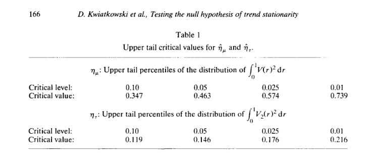
The problem is that the statistical packages (statsmodels.tsa.stattools.kpss in python and kpss.test in R) report p=0.01 if the test statistic is above the critical threshold. They don't report p-values below 0.01. The thresholds are given in the original paper: Kwiatkowski, D.; Phillips, P. C. B.; Schmidt, P.; Shin, Y. (1992). "Testing the null hypothesis of stationarity against the alternative of a unit root".

The test distribution is non-standard. Does anyone have an idea how to do this? I imagine I can follow the original paper and compute new critical values for my adjusted significance, but that would be a lot of work. Anyone encountered this problem before? Or know a quick way to adjust the p-values?

The critical values for $\alpha=0.001$ is 1.16786, according to Nabeya, Seiji, and Katsuto Tanaka. "Asymptotic theory of a test for the constancy of regression coefficients against the random walk alternative." The Annals of Statistics (1988): 218-235. This was also cited in the Kwiatkowski et al paper.

Answer 1

You are correct that the null distribution is nonstandard. In the level case, it is (cf. KPSS's eq. (14)) the integral over a squared Brownian Bridge $$ \int_0^1(W(r)-rW(1))^2dr $$ Fortunately, such a functional is not too difficult to simulate - and it would therefore arguably indeed be a good idea to incorporate this in the said packages (see also How is the augmented Dickey–Fuller test (ADF) table of critical values calculated?):

n <- 10000

squared.BrownianBridge <- function(n){
  W <- n^(-1/2)*cumsum(rnorm(n))
  r <- seq(0, 1, length=n)
  V <- W - r*W[n]
  mean(V^2)  
}

squared.BB.dist <- replicate(50000, squared.BrownianBridge(n))

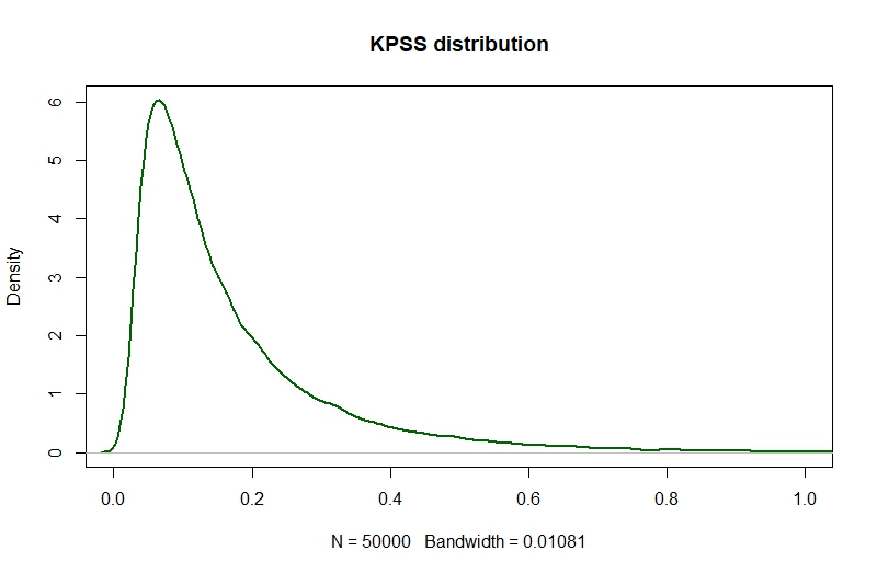
The distribution looks like this (the slight support on negative values is an artefact from using density to estimate the distribution from the draws):

You can check that it returns the right (up to simulation variability) critical values from the upper panel of Table 1 in KPSS from invoking:

quantile(squared.BB.dist, probs=c(0.9, 0.95, 0.975, 0.99, 0.999))

      90%       95%     97.5%       99%     99.9% 
0.3477930 0.4659657 0.5871195 0.7512138 1.1727415 

Now, we store the empirical cdf and can evalaute (since it is a right-tailed test) p-values given your values of the test statistic as follows:

squared.BB.dist.ecdf <- ecdf(squared.BB.dist)
someteststat <- 0.5
p.value <- 1-squared.BB.dist.ecdf(someteststat)

The $m$ $p$-values computed in this way may now as usual be compared against the Bonferroni threshold $\alpha/m$ (or of course thresholds of any other, possibly more powerful multiple testing procedure based on $p$-values).

Extension:

The lower panel of Table 1 for the trend case requires simulating (cf. eq. (18)) $$ \int_0^1\left[W(r) + (2r-3r^2)\cdot W(1)+(-6r+6r^2)\int_0^1W(s)ds\right]^2dr $$ like so:

squared.BrownianBridge.trend <- function(n){
  W <- n^(-1/2)*cumsum(rnorm(n))
  r <- seq(0, 1, length=n)
  V.2 <- W + (2*r-3*r^2)*W[n]+(-6*r+6*r^2)*mean(W)
  mean(V.2^2)  
}

squared.BB.dist.trend <- replicate(50000, squared.BrownianBridge.trend(n))
quantile(squared.BB.dist.trend, probs=c(0.9, 0.95, 0.975, 0.99, 0.999))