What is the relationship between the Brier score "refinement" and the area under the ROC curve?

Question

In the Wikipedia article on Brier score, there is a claim that the "refinement" in the two-component decomposition of Brier score is related to the area under the receiver-operator characteristic curve (itself equal to Harrell's concordence index in the case of a binary outcome).

What is that relationship? A simlation of mine makes it look like there is a slight difference between the two, and and this Cross Validated question/self-answer makes it look like there can be disagreement.

From the phrasing on Wikipedia, I would expect an explicit relationship between refinement and ROCAUC the way that ROCAUC and Somers' $D_{xy}$ can be related by $D_{xy} = 2ROCAUC - 1$. Is there such a function mapping between refinement and ROCAUC, particularly a bijective function?

library(SpecsVerification)
library(pROC)
library(ggplot2)
set.seed(2023)
N <- 1000
R <- 1000
p <- rbeta(N, 1/4, 1/4)
y <- rbinom(N, 1, p)

SpecsVerification::BrierDecomp(p, y)#[1, 1]
res <- function(y, p){
  return(SpecsVerification::BrierDecomp(p, y)[1, 2])
}
cal <- rel <- function(y, p){
  return(SpecsVerification::BrierDecomp(p, y)[1, 1])
}
unc <- function(y, p){
  return(SpecsVerification::BrierDecomp(p, y)[1, 3])
}
ref <- function(y, p){

  brier <- mean((y - p)^2)
  return(brier - cal(y, p))

}

# Do the loops
#
rocs <- refs <- rep(NA, R)
for (i in 1:R){

  p <- rbeta(N, 1, 1)
  y <- rbinom(N, 1, p)
  
  rocs[i] <- pROC::roc(y, p)$auc
  refs[i] <- ref(y, p)
  
  if (i < 5 | i %% 75 == 0){
    print(paste(
      i/R*100, "% complete", sep = ""
    ))
  }
  
  
}
d <- data.frame(rocs, refs)
ggplot(d, aes(x = rocs, y = refs)) +
  geom_point() +
  xlab("ROCAUC") +
  ylab("Refinement")

There is a huge correlation in the expected direction in this simlation. However, the relationship is not perfectly monotonic. What gives? Is it just some rounding that causes the imperfect correlation? Is the relationship between refinement and ROCAUC considerable but not supposed to be perfect? Does the relationship only converge to a perfect correlation as the sample size tends toward infinity?

Answer 1

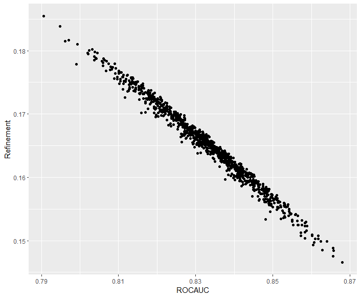
This inclusion on the wiki article occurred without any citations. It is not wrong, per se. If sharpness is 0 (resolution equal to uncertainty), then AUC is 0 or 1. If sharpness (refinement) is equal to uncertainty (no resolution), then the AUC is 0.5.

Other than that, it is not possible to further relate both quantities.

I tried to bring the formulas together below to identify perhaps boundaries that could be expressed in terms of either without success. I believe my discrete version of the AUC is correct now (after some edits), but let me know if anything is not clear.

Sharpness can be expressed, assuming a number $K$ of discrete probabilities are issued, as:

\begin{align} \text{Sharpness} &= E[(X-E[X|P])^2] = \frac{1}{N}\sum_{i=1}^{K} \sum_{j=1}^{N_i} (x_{ij} - \bar x_i)^2\\ &= \frac{1}{N}\sum_{i=1}^{K} {N_i} \frac{N_i^+}{N_i} (1 - \bar x_i)^2 + {N_i}\frac{N_i^-}{N_i} \bar x_i^2 \frac{1}{N}\sum_{i=1}^{K} {N_i} \bar x_i (1 - \bar x_i)^2 + {N_i}(1 - \bar x_i) \bar x_i^2 = \\ &= \frac{1}{N}\sum_{i=1}^{K} {N_i} \bar x_i (1 - \bar x_i) \end{align}

$\bar x_i$ is the expected output in a given probability forecast, $x_{ij}$ represents the real outcome in example $j$ of the $i$-th probability forecast level. ${N_i}$ is the number of examples that are issued the $i$-th probability forecast level, and ${N_i}^+$ and ${N_i}^-$ are respectively the number of positive and negative examples at this particular forecast.

We can show that (see this answer)

\begin{align} \text{AUC} &= \int_0^1 \operatorname{TPR}(\operatorname{FPR}) d\operatorname{FPR}\\ &= \int_0^1 \operatorname{TPR}(\operatorname{FPR}(\tau)) d\operatorname{FPR}(\tau) \\ &= \int_{+\infty}^{-\infty} \operatorname{TPR}(\tau) \operatorname{FPR}'(\tau) d\tau \\ &= \int_{+\infty}^{-\infty} \big( 1-F_1(\tau) \big) \big( -f_0(\tau) \big) d\tau \\ &= \int_{-\infty}^{+\infty} \big( 1-F_1(\tau) \big) f_0(\tau) d\tau \\ &= \int_{-\infty}^{+\infty} f_0(\tau) d\tau - \int_{-\infty}^{+\infty} F_1(\tau) f_0(\tau) d\tau \\ &= 1 - \int_{-\infty}^{+\infty} \int_{-\infty}^{\tau}f_1(\tau') f_0(\tau) d\tau' d\tau \\ &= 1 - \int_{-\infty}^{+\infty} f_0(\tau) \int_{-\infty}^{\tau}f_1(\tau') d\tau' d\tau \\ \end{align}

Assuming again discrete probabilities for the AUC, we can write

$$ \begin{align} \text{AUC} &= 1 - \frac{1}{N^-N^+}\sum_{i=1}^{K} N_i^- \sum_{j=1}^{i} N_j^+\\ &=1 - \frac{1}{N^2 \bar x (1 - \bar x)}\sum_{i=1}^{K} N_i \frac{N_i^-}{N_i} \sum_{j=1}^{i} N_j \frac{N_j^+}{N_j} = \\ &=1 - \frac{1}{N^2 \bar x (1 - \bar x)}\sum_{i=1}^{K}\sum_{j=1}^{i} N_i N_j \bar x_j (1 - \bar x_i) = \\ &=1 - \sum_{i=1}^{K}\sum_{j=1}^{i} \frac{N_i N_j}{N^2} \frac{\bar x_j (1 - \bar x_i) }{\bar x (1 - \bar x)} = \\ &=1 - \sum_{i=1}^{K} \frac{N_i^2}{N^2} \frac{\bar x_i (1 - \bar x_i)}{\bar x (1 - \bar x)} - \sum_{i=2}^{K}\sum_{j=1}^{i-1} \frac{N_i N_j}{N^2} \frac{\bar x_j (1 - \bar x_i) }{\bar x (1 - \bar x)}\\ \end{align} $$

If we assume $\bar x_i=\bar x$

$$ \begin{align} \text{AUC} &=1 - \sum_{i=1}^{K}\sum_{j=1}^{i} \frac{N_i N_j}{N^2} \frac{\bar x (1 - \bar x)}{\bar x (1 - \bar x)}\\ &=1 - \sum_{i=1}^{K}\sum_{j=1}^{i} \frac{N_i N_j}{N^2}\\ \end{align} $$

We can show that

$$N^2=\left(\sum_{i=1}^{K}N_i\right)^2=2\sum_{i=1}^{K}\sum_{j=1}^{i}N_iN_j$$

Thus

$$ \begin{align} \text{AUC} &=1 - \sum_{i=1}^{K}\sum_{j=1}^{i} \frac{N_i N_j}{N^2}\\ \end{align} =1-\frac{1}{2}\frac{N^2}{N^2}=0.5, $$

and $$ \begin{align} \text{Sharpness} &= \frac{1}{N}\sum_{i=1}^{K} {N_i} \bar x_i (1 - \bar x_i) = \frac{1}{N}\sum_{i=1}^{K} {N_i} \bar x (1 - \bar x)\\ &= \bar x (1 - \bar x)\sum_{i=1}^{K} \frac{N_i}{N}= \bar x (1 - \bar x)=\text{Uncertainty} \end{align} $$

If we assume $\bar x_i \in \{0,1\}$

$$ \begin{align} \text{Sharpness} &= \frac{1}{N}\sum_{i=1}^{K} {N_i} \bar x_i (1 - \bar x_i) = 0 \end{align} $$

This is the perfect Sharpness score, where the Uncertainty is negated by the forecast Resolution. On the other hand,

$$ \begin{align} \text{AUC} &=1 - \sum_{i=1}^{K}\sum_{j=1}^{i} \frac{N_i N_j}{N^2} \frac{\bar x_j (1 - \bar x_i) }{\bar x (1 - \bar x)}\\ &=1 - \sum_{i=2}^{K}\sum_{j=1}^{i-1} \frac{N_i N_j}{N^2} \frac{\bar x_j (1 - \bar x_i) }{\bar x (1 - \bar x)}\\ \end{align} $$

Here, we have to further assume that there is an index $i'$ for which $\bar x_{i}=1 ~\forall~ i>i', 1\lt i' \lt K$, $\bar x_i = 0$ otherwise. This is where the intrinsic ordering of the scores shows up in the perfect AUC score.

With that assumption, we can split the sums, once for each index,

$$ \begin{align} \text{AUC} &=1 - \sum_{i=2}^{i'}\sum_{j=1}^{i-1} \frac{N_i N_j}{N^2} \frac{\bar x_j \cdot (1 - \overbrace{0}^{\bar x_i=0~\forall~i\leq i'})}{\bar x (1 - \bar x)} - \overbrace{\sum_{i=i'+1}^{K}\sum_{j=1}^{i-1} \frac{N_i N_j}{N^2} \frac{\bar x_j \cdot (1 - 1)}{\bar x (1 - \bar x)}}^{=0~\because~ \bar x_i=1~\forall~i\gt i'}\\ &=1 - \sum_{i=2}^{i'}\sum_{j=1}^{i-1} \frac{N_i N_j}{N^2} \frac{\overbrace{\bar x_j}^{=0~\because~j<i\leq i'}}{\bar x (1 - \bar x)}=1 \end{align} $$

Similarly, assuming instead that here is an index $i'$ for which $\bar x_{i}=1 ~\forall~ i\leq i', 1\lt i' \lt K$, $\bar x_i = 0$ otherwise, we once again can split the sums,

$$ \begin{align} \text{AUC} &=1 - \overbrace{\sum_{i=2}^{i'}\sum_{j=1}^{i-1} \frac{N_i N_j}{N^2} \frac{\bar x_j \cdot (1 - 1)}{\bar x (1 - \bar x)}}^{=0~\because~ \bar x_i=1~\forall~i\leq i'} - \sum_{i=i'+1}^{K}\sum_{j=1}^{i-1} \frac{N_i N_j}{N^2} \frac{\bar x_j \cdot (1 - 0)}{\bar x (1 - \bar x)}\\ &=1 - \sum_{i=i'+1}^{K}\sum_{j=1}^{i'} \frac{N_i N_j}{N^2} \frac{\overbrace{(1) }^{\bar x_j=1~\because~j\leq~i'}}{\bar x (1 - \bar x)} - \sum_{i=i'+2}^{K}\sum_{j=i'+1}^{i-1} \frac{N_i N_j}{N^2} \frac{\overbrace{(0)}^{\bar x_j=0~\because~j\gt~i'}}{\bar x (1 - \bar x)}\\ &=1 - \sum_{i=i'+1}^{K}\sum_{j=1}^{i'} \frac{N_i N_j}{N^2} \frac{1}{\bar x (1 - \bar x)} =1 - \frac{\left(\sum_{i=i'+1}^{K} N_i\right) \left(\sum_{j=1}^{i'}N_j\right)}{N^2 \bar x (1 - \bar x)}\\ \end{align} $$

Due to the intrinsic ordering we introduced

$$\sum_{i=i'+1}^{K}N_i=\bar xN$$

is the total number of positives examples and, similarly,

$$\sum_{j=1}^{i'}N_j=(1-\bar x)N$$

is the sum of all negative examples. Thus

$$ \begin{align} \text{AUC} &=1 - \frac{\left(\sum_{i=i'+1}^{K} N_i\right) \left(\sum_{j=1}^{i'}N_j\right)}{N^2 \bar x (1 - \bar x)} &=1-\frac{N^2\bar x(1-\bar x)}{N^2 \bar x (1 - \bar x)}=0 \end{align} $$

This way we show that perfectly separated classes per bin will result in $\text{Sharpness}=0$ and $\text{AUC}=0$ or $\text{AUC}=1$, depending on the orientation of the scores.