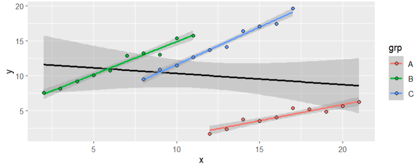
I'm new to the world of mixed-effects models and trying to understand what method/results to report for my given data/question. I am trying to determine the coefficients of a regression model but have three sub-populations within the data. My question is 1) whether y is predicted from x at a likelihood much greater than chance and 2) whether the slope is essentially the same for each sub-population. I've simulated some data that shows this:
set.seed(123)
dat <- data.frame(grp=gl(3, 10, labels = LETTERS[1:3]))
dat$y <- 1:10+as.numeric(dat$grp)*3
dat$x <- 1:10+as.numeric(dat$grp)[rep(c(1,3,2), each=10)]
dat$x <- ifelse(dat$grp=="A", dat$x+10, dat$x)
dat$x <- ifelse(dat$grp=="C", dat$x+6, dat$x)
dat$y <- ifelse(dat$grp=="A", dat$y*0.5, dat$y)
dat$y <- dat$y+rnorm(30, sd = 0.5)

library(ggplot2)
ggplot(dat, aes(x=x, y=y)) +
  geom_smooth(color="black", method="lm") +
  geom_smooth(aes(color=grp), method="lm") +
  geom_point(aes(fill=grp), pch=21)
Visually (and correctly, given that this data is simulated) the answers to my questions are relatively simple: yes, y is predicted from x, and kinda, with B ~ C > A. The question is how I should best show this statistically and what I should report for my actual data.
Obviously the overall (black) trend is incorrect and is an illustration of Simpson's paradox, so I'll ignore it entirely. The ggplot lines are fit independently to each sub-population with a basic call to lm that I can reproduce with a simple loop. These values then need to be corrected for multiple comparisons and I do so separately for the slopes and intercepts since I want to keep the FWER distinct for each.
loop_vals <- do.call(rbind, lapply(unique(dat$grp), function(grp_i){
  broom::tidy(lm(y~x, data=dat[dat$grp==grp_i,]))
}))
p.adj <- c(p.adjust(loop_vals$p.value[c(1,3,5)]), p.adjust(loop_vals$p.value[c(2,4,6)]))
loop_vals$p.adj <- p.adj[c(1,4,2,5,3,6)]
  term        estimate std.error statistic      p.value        p.adj
  <chr>          <dbl>     <dbl>     <dbl>        <dbl>        <dbl>
1 (Intercept)   -3.29     0.901      -3.65 0.00650      0.0130
2 x              0.459    0.0538      8.54 0.0000273    0.0000273
3 (Intercept)    5.52     0.399      13.8  0.000000722  0.00000217
4 x              0.936    0.0562     16.7  0.000000171  0.000000342
5 (Intercept)    0.879    0.614       1.43 0.190        0.190
6 x              1.07     0.0479     22.4  0.0000000167 0.0000000501
I can obtain these same values with an interaction-based model in a single call to lm(), but the significance values are wildly different (or I don't understand how the error propagates differently here). This likely just has to do with multiple comparisons?
broom::tidy(lm(y~x*grp, data=dat))
  term        estimate std.error statistic       p.value
  <chr>          <dbl>     <dbl>     <dbl>         <dbl>
1 (Intercept)   -3.29     0.883      -3.72 0.00106
2 x              0.459    0.0527      8.70 0.00000000686
3 grpB           8.81     0.959       9.18 0.00000000253
4 grpC           4.17     1.11        3.74 0.00100
5 x:grpB         0.477    0.0746      6.39 0.00000131
6 x:grpC         0.614    0.0746      8.23 0.0000000191
Alternatively, I can fit the data using a mixed effects model. Fitting this with random intercepts and fixed slopes gives reasonable results and an easily interpretable output, but I've heard mixed advice on trying to model a random effect with so few groups (less than 5):
lme_fixed_slope_mod <- lme4::lmer(y~x+(1|grp), data=dat, REML = FALSE)
Random effects:
 Groups   Name        Std.Dev.
 grp      (Intercept) 6.8323
 Residual             0.9156
Number of obs: 30, groups:  grp, 3
Fixed Effects:
(Intercept)            x
     0.3904       0.8171
Finally, I can fit the data with random slopes and random intercepts. I've been told this is generally a good idea but worry that it won't answer my overall question about the slope estimate as clearly. Doing this returns predictions that are very similar to (but distinct from!) the values obtained from the lm outputs above, and I can't figure out how to extract the slopes and intercepts themselves from the lmerMod object. I expected these predictions to be the same as the lm models and don't understand why they're different.
lme_rand_slope_mod <-lme4::lmer(y~x+(1+x|grp), data=dat, REML = FALSE)
Random effects:
 Groups   Name        Std.Dev. Corr
 grp      (Intercept) 3.6281
          x           0.2571   0.77
 Residual             0.4778
Number of obs: 30, groups:  grp, 3
Fixed Effects:
(Intercept)            x
     1.1102       0.8192
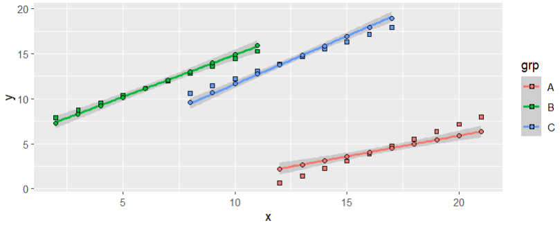
Comparison of the three slope/intercept values (boxes = fixed slope, circles = random). Note that while the circles appear to fall right on the line of best fit, they're actually deviating systematically.
dat$y_lmpred <- predict(lm_model, newdata=dat[,c("x", "grp")])
dat$y_lme_fixedpred <- predict(lme_fixed_slope_mod, newdata=dat[,c("x", "grp")])
dat$y_lme_randpred <- predict(lme_rand_slope_mod, newdata=dat[,c("x", "grp")])

ggplot(dat, aes(x=x, y=y)) +
  geom_smooth(aes(color=grp), method="lm") +
  geom_point(aes(x=x, y=y_lme_fixedpred, fill=grp), shape=22) +
  geom_point(aes(x=x, y=y_lme_randpred, fill=grp), shape=21)
Which of these four methods is most apt for my data and will help me answer 1) whether x is a good predictor of y and 2) whether the slopes are indistinguishable for the subgroups in my real data set? What values should I report to show this?


