Get unbiased derivative from GAM

Question

I have time-dependent data and I'm interested in the gradient at time zero. From theory I expect the gradient of the true relationship to be highest at time zero.

I would like to estimate the derivative at time zero using a GAM. However, the estimates are biased (too low). How can I reduce or preferably eliminate that bias?

#HM function
HM <- function(t, f0, phi, kappa) phi + f0 * exp(-kappa * t)/(-kappa)

t <- 0:180
phi <- 530
kappa <- 0.025
f0 <- 5
Ctrue <- HM(t, f0, phi, kappa)

sdC <- 5

library(mgcv)
library(gratia)

set.seed(1)
res <- replicate(100, {
  
  C <- Ctrue + rnorm(length(t), sd = sdC)
  
  DF <- data.frame(C, t)
  
  
  fit <- gam(C ~ s(t, bs = "bs", k = 5), data = DF)
  #gam.check(fit)
  
  #ggplot(DF, aes(t, C)) +
  #  geom_point() +
  #  stat_function(fun = \(t) predict(fit, newdata = data.frame(t)))
  
  derivatives(fit, data = data.frame(t = 0))
  
}, simplify = FALSE)

res <- do.call(rbind, res)

summary(res$derivative)
# Min. 1st Qu.  Median    Mean 3rd Qu.    Max. 
#4.266   4.432   4.508   4.517   4.589   4.773

#True value is 5

Answer 1

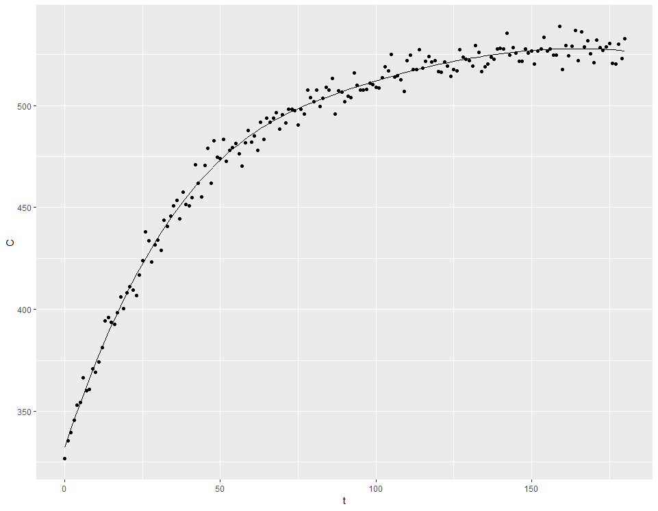
I suggest you may need to increase the potential complexity of the basis (i.e. increase k) and perhaps even extend the range of the penalty beyond zero to get more accurate and correct estimates of the slope at t = 0. I used your same data-generating process and, with these modifications, got a better answer (note that I'm using {marginaleffects} for these calculations, but I'm certain you could do this just as well with {gratia}:

library(mgcv)
library(marginaleffects)
library(ggplot2)
theme_set(theme_bw())

#HM function
HM <- function(t, f0, phi, kappa) phi + f0 * exp(-kappa * t)/(-kappa)

set.seed(1)
t <- 0:180
phi <- 530
kappa <- 0.025
f0 <- 5
Ctrue <- HM(t, f0, phi, kappa)
sdC <- 5
C <- Ctrue + rnorm(length(t), sd = sdC)
DF <- data.frame(C, t)

# The model
fit <- gam(C ~ 
             # Use larger 'k' for more flexibility, 
             # particularly near the endpoints
             s(t, bs = "bs", k = 10),
           
           # Extend penalty beyond zero for more effective 
           # estimates of derivatives at the bound
           knots = list(t = c(-5, 0, 180, 185)),
           data = DF)
#> Warning in smooth.construct.bs.smooth.spec(object, dk$data, dk$knots): there is
#> *no* information about some basis coefficients

# The estimated function, on the response scale
plot_predictions(fit, condition = 't',
                 points = 0.5)

# Estimated slopes (using a finer grid of points for a smoother image)
plot_slopes(fit, 
            newdata = datagrid(t = seq(0, 180, by = 0.2)),
            variables = 't', by = 't')

# Estimated slope at t = 0, with appropriate uncertainty envelope
slopes(fit, 
       newdata = datagrid(t = seq(0, 180, by = 0.2)),
       variables = 't', by = 't')[1,]
#> 
#>  Term    Contrast t Estimate Std. Error  z Pr(>|z|)     S 2.5 % 97.5 %
#>     t mean(dY/dX) 0     4.72      0.336 14   <0.001 146.0  4.06   5.38
#> 
#> Columns: rowid, term, contrast, t, estimate, std.error, statistic, p.value, s.value, conf.low, conf.high, predicted_lo, predicted_hi, predicted 
#> Type:  response

# Does the estimate at t = 0 differ 'significantly' from 5?
hypotheses(slopes(fit, 
                  newdata = datagrid(t = seq(0, 180, by = 0.2)),
                  variables = 't', by = 't'),
           hypothesis = 5)[1,]
#> 
#>  Term    Contrast t Estimate Std. Error      z Pr(>|z|)   S 2.5 % 97.5 %
#>     t mean(dY/dX) 0     4.72      0.336 -0.841      0.4 1.3  4.06   5.38
#> 
#> Columns: rowid, term, contrast, t, estimate, std.error, statistic, p.value, s.value, conf.low, conf.high, predicted_lo, predicted_hi, predicted 
#> Type:  response

^{Created on 2024-03-25 with reprex v2.1.0}

You can read more about how the penalty can be extended in this way using b-splines in Gavin Simpson's helpful post on spline extrapolation