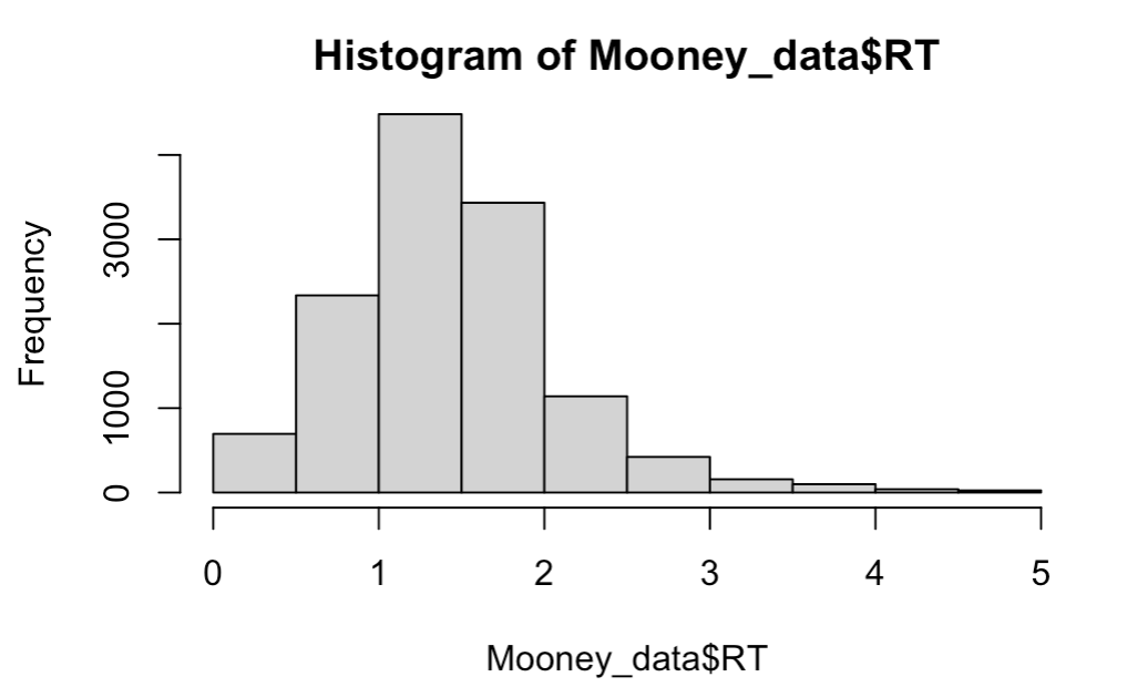
I am examining the effect of 'Phase' on reactions time (RT) data using a mixed model in lme4.
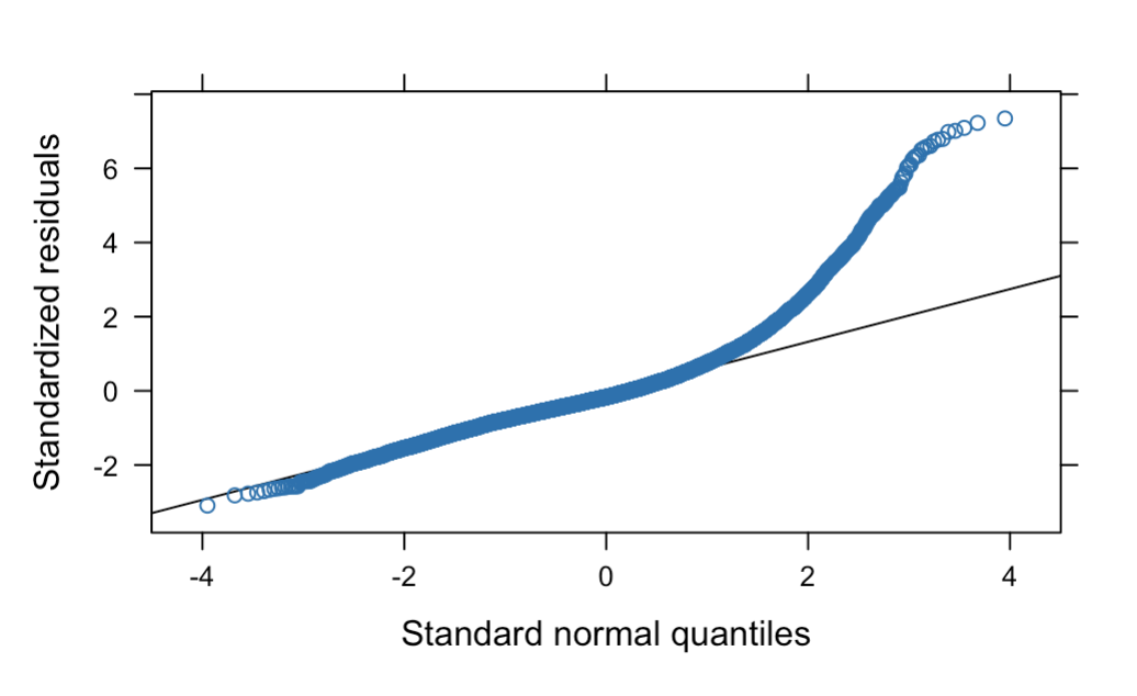
However, as is common with RT data, the residuals are non-normal.
This is the first model, which is a linear mixed model approach:
RT_lme<- lmer(RT ~ Phase.ct + (Phase.ct|Pt_ID) + (Phase.ct|Image),
data = Mooney_data, control=lmerControl(optimizer="bobyqa"))

summary(RT_lme)

Fixed effects:
            Estimate Std. Error       df t value Pr(>|t|)
(Intercept)  1.44591    0.04533 80.20875  31.897   <2e-16 ***
Phase.ct     0.02967    0.01624 72.24639   1.827   0.0718 .
Figure 1 plot shows the non-normality problem.
As I realise that transforming RT data is not recommended, I followed the methods using in the paper by Lo & Andrews (2015). See here: https://www.frontiersin.org/journals/psychology/articles/10.3389/fpsyg.2015.01171/full#h8
I therefore fit the following 2 generalised linear mixed models, which use different link functions:
1.
RT_lme1<- glmer(RT ~ Phase.ct + (Phase.ct|Pt_ID) + (Phase.ct|Image),
data = Mooney_data,family=Gamma(link=invfn()),control=glmerControl(optimizer="bobyqa"))

summary(RT_lme1)

Fixed effects:
            Estimate Std. Error t value Pr(>|z|)
(Intercept) -778.393      8.627 -90.225  < 2e-16 ***
Phase.ct      22.547      8.098   2.784  0.00536 **
-
RT_lme2<- glmer(RT ~ Phase.ct + (1|Pt_ID),data = Mooney_data,family=inverse.gaussian(link=invfn()),control=glmerControl(optimizer="bobyqa"))
summary(RT_lme2)
Fixed effects: Estimate Std. Error t value Pr(>|z|)
(Intercept) -736.62 12.71 -57.953 < 2e-16 *** Phase.ct 16.61 6.34 2.621 0.00877 **
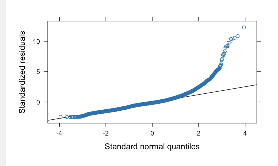
However, both plots still show that the residuals are non-normal (example below). I have limited understanding of how altering the link function affects the model. Would this be expected to reduce non-normality? How do I select the best model (I thought to use AIC values but am concerned about non-normality in the plots)?


