I have some animal species. I am interested in seeing what is the relationship between the area they occupy (my response variable, p, which is a count of cells) and my independent variables (e.g., human population density PopdensityAvg_3035_average). I have some outliers which I cannot discard, because I am interested in these extreme values. I suppose there is a difference in how each species behaves, and how each species will specifically respond to different types of land-use, thus I include a random intercept for species (Binomial) and also a random slope for land-use (landuseHAvg_3035_average). I decided to use a negative binomial distribution with offset (log of POAR) instead of other distributions, because each area of a species (p) cannot be wider than the total area (POAR). My model formula using glmmTMB v.1.1.8 in R looks like:
mod <- glmmTMB(get(p) ~ Pathways_tot + Native_range +
        PopdensityAvg_3035_average  + landuseHAvg_3035_average +
        infrastructuresAvg_3035_average + offset(log(POAR)) +
         (landuseHAvg_3035_average | Binomial),
        control = glmmTMBControl(optimizer = optim,
        optArgs = list(method = "L-BFGS-B")), data = df,
                       family = nbinom2)

summary(mod)

Family: nbinom2  ( log )
Formula:          get(p) ~ Pathways_tot + Native_range +
  PopdensityAvg_3035_average +      landuseHAvg_3035_average +
  infrastructuresAvg_3035_average +
    offset(log(POAR)) + (landuseHAvg_3035_average | Binomial)
Data: df

     AIC      BIC   logLik deviance df.resid
  7963.4   8013.0  -3971.7   7943.4     1040

Random effects:

Conditional model:
 Groups   Name                     Variance Std.Dev. Corr
 Binomial (Intercept)              2.014    1.419
          landuseHAvg_3035_average 2.139    1.462    -0.61
Number of obs: 1050, groups:  Binomial, 33

Dispersion parameter for nbinom2 family (): 0.321

Conditional model:
                                Estimate Std. Error z value             Pr(>|z|)
(Intercept)                      -4.0862     0.5458  -7.487   0.0000000000000704 ***
Pathways_tot                     -0.3730     0.2099  -1.777               0.0756 .
Native_range                     -0.2376     0.2065  -1.151               0.2499
PopdensityAvg_3035_average        2.1589     0.0989  21.830 < 0.0000000000000002 ***
landuseHAvg_3035_average         -0.4937     0.3323  -1.486               0.1374
infrastructuresAvg_3035_average  -0.6032     0.1032  -5.846   0.0000000050314892 ***
---
Signif. codes:  0 ‘***’ 0.001 ‘**’ 0.01 ‘*’ 0.05 ‘.’ 0.1 ‘ ’ 1
The values of deviance and degrees of freedom are very different. I check for over-/under-dispersion with DHARMA v.0.4.6:
testDispersion(mod)

    DHARMa nonparametric dispersion test via sd of residuals fitted vs. simulated

data:  simulationOutput
dispersion = 0.00006321, p-value = 0.016
alternative hypothesis: two.sided
I get the same result with performance v.0.11.0:
check_overdispersion(mod)
# Overdispersion test

 dispersion ratio = 0.000
          p-value = 0.016

Underdispersion detected.
However, in ?check_overdispersion I read:
Using this approach would be inaccurate for zero-inflated or negative binomial mixed models (fitted with glmmTMB). In such cases, the overdispersion test is based on simulate_residuals() (which is identical to check_overdispersion(simulate_residuals(model))).
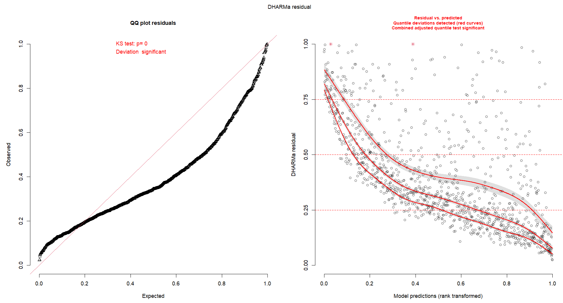
plot(simulateResiduals(fittedModel = mod)) returns the following:
But I get a message:
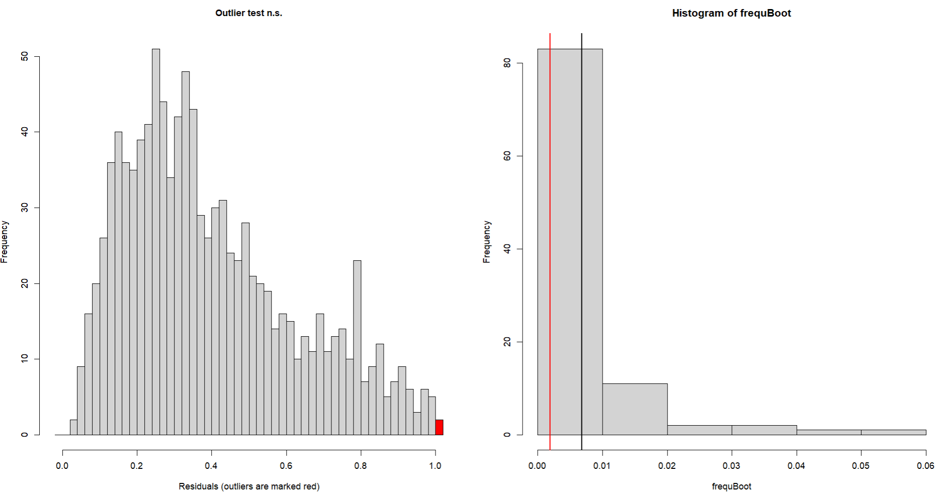
DHARMa:testOutliers with type = binomial may have inflated Type I error rates for integer-valued distributions. To get a more exact result, it is recommended to re-run testOutliers with type = 'bootstrap'. See ?testOutliers for details
testOutliers(mod, type = 'bootstrap')

    DHARMa bootstrapped outlier test

    data:  mod
    outliers at both margin(s) = 2, observations = 1050,
    p-value = 0.68
    alternative hypothesis: two.sided
     percent confidence interval:
     0.00000000 0.03347619
    sample estimates:
    outlier frequency (expected: 0.00678095238095238 )
                                           0.001904762
I know I have few outliers but, again, I would be interested in keeping them. So far I am not seeing other strong problems. This model is one of a set of 3, all of them rely on the same assumptions and what changes are the areas occupied (different proportions of the total area available). Apart from the DHARMA message on outliers, I don't get any other message. As far as I've seen so far (e.g., GLMM FAQ), procedures to to deal with under-dispersion are similar to those for over-dispersion, including switching distribution. Based on my data, however, i think negative binomial may be appropriate. Lastly, for what I've read, as under-dispersion is more conservative, it is seen as a minor problem (compared to over-).
My question is: shall I try (and if yes, how?) to address under-dispersion or outliers problems?


