2
$\begingroup$

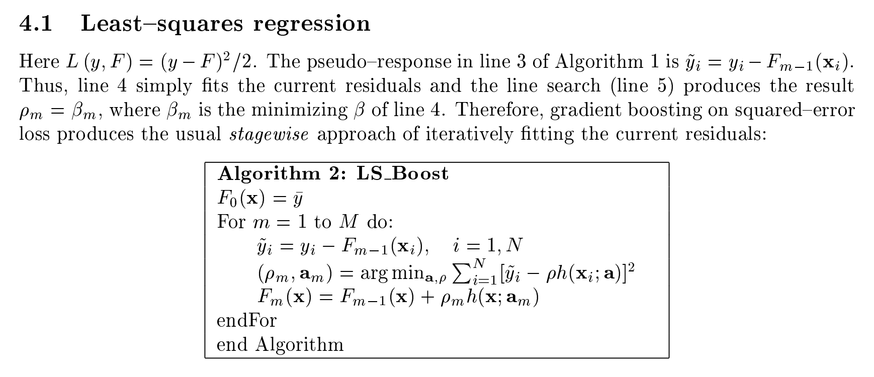
I have recently done some work altering popular gradient boosted decision trees (GBDTs) for regression, and I was just working on establishing a theoretic basis for the modern algorithm. There is a paper here I've gravitated toward from Jerome Friedman (1999): Greedy Function Approximation: A Gradient Boosting Machine. There is a nice background developed in the intro, and I've found what I think is the general algorithm for GBDTs for regression, copied here, Algorithm 2.

LS Boost

My question is going to become apparent now. Inside the for loop we have three lines. The first line is simply computing the gradients based on the stagewise learner until that step. The $h(\textbf{x},\textbf{a})$ is the parametrized function (regression tree) that is fit to the residuals at each stage. This fitting is happening on the second line. On this line the parameter $\rho_m$ is also being optimized, which is then used in the last step to scale the update to the function $F$.

The way I interpret $\rho_m$ is what we now call the learning rate in popular GBDT libraries like XGBoost or LightGBM. $\rho_m$ is set as a fixed value at the beginning of training, it is not optimized for at each step like in this algorithm. Why is that? Is there an important paper that discusses why this simplification is made? This algorithm makes it seem that we should adjust the learning rate at each stage instead of keeping it fixed. I'm just wondering why we seem to have lost this detail with modern GBDT implementations?

$\endgroup$
1
  • 2
    $\begingroup$ I can't speak to the historical development, but I tend to think of the learning rate as providing additional regularization (setting it closer to 0 than to 1), whereas I would expect the optimal $\rho_m$ to be close to 1 at most boosting stages. And I wouldn't expect much lift in the training fit by optimizing, at the cost of performing that optimization. $\endgroup$ Commented May 29 at 18:39

1 Answer 1

3
$\begingroup$

Going to 'slow learning' was not a simplification, it was an improvement. The value $\rho_m$ in the earlier algorithm is a greedy optimal coefficient for the current weak learner, but in the context of the whole fitting procedure it tends to be too large. Reducing it improves the fit (at the cost of more rounds and thus more computation).

Using a small value for $\rho_m$ gives something close to L1-regularisation, and allows more features to contribute to the predictor. This is all tidiest in the setting where the stagewise learners are simple linear regressions. The greedy optimal $\rho_m$ then gives forward stagewise regression and sufficiently small $\rho_m$ gives least angle regression (or, with slight adjustments, the lasso). Two references are the Least Angle Regression paper and Chapter 10 of Elements of Statistical Learning by Hastie, Friedman, and Tibshirani.

I don't think that group were the even close to the first to realise that 'slow learning' gave improved results, but I do think they were the first to make precise the relationship to L1-regularisation. I learned this stuff from talks given by Tibshirani and Hastie in the early 2000s.

$\endgroup$

Your Answer

By clicking “Post Your Answer”, you agree to our terms of service and acknowledge you have read our privacy policy.

Not the answer you're looking for? Browse other questions tagged or ask your own question.